

RF PA efficiency changes a C-UAS project’s DC load and waste-heat budget. Whether it lowers five-year TCO depends on the power supplies, cooling equipment and operating hours the project actually needs. Compare RF power amplifier efficiency and system cost only between candidates that meet the same RF task, with efficiency measured at equivalent boundaries and
operating conditions.
Lower DC draw may permit a smaller power supply or different cooling arrangement. If both candidates fit the same hardware, those purchase costs may stay unchanged. Price the downstream consequences before accepting an amplifier premium.
1. Which RF PA Efficiency Figures Can Be Used for System Cost Comparison?
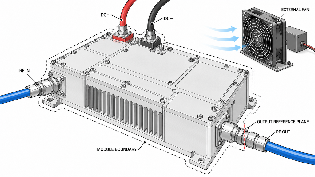
The efficiency figure must describe the same amplifier boundary that the buyer intends to power. For the illustrative calculations below, module DC-to-RF efficiency is net RF output power at the defined PA output reference plane divided by DC input power measured at the module’s DC terminals:
η_module = Pout / Pdc
The module’s DC total must include every DC feed crossing that boundary, including supplies for internal auxiliaries. Power for external drivers, controllers or fans belongs elsewhere in the system budget; it must neither disappear nor be counted twice. Where load mismatch is material, suppliers must distinguish forward power from net delivered output and report forward/reverse measurements corrected to the stated reference plane.
Module DC-to-RF efficiency, power-added efficiency (PAE = (Pout − Pin) / Pdc) and transistor drain efficiency measure different things. RF drive and auxiliary consumption affect the result. A reported 45% PAE for one device cannot be ranked directly against 40% drain efficiency for another. The definitions and drive boundary in PAE verification before an RFQ clarify which figures belong in the DC budget.
Both candidates must meet the same frequency, net PA-port output, waveform, duty cycle, load or VSWR condition, supply voltage and hot operating state. Record the measurement reference planes and whether each figure is nominal or measured. A peak-efficiency figure taken at a different output or temperature is insufficient; request module DC input data under matched conditions. Screen for technical suitability using C-UAS RF amplifier module selection before comparing costs.
2. How Does PA Efficiency Change DC Power and Heat Load?
With comparable module efficiencies, calculate DC watts, terminal current and waste heat at the specified RF output:
Pdc = Pout / η_module; Idc = Pdc / Vdc
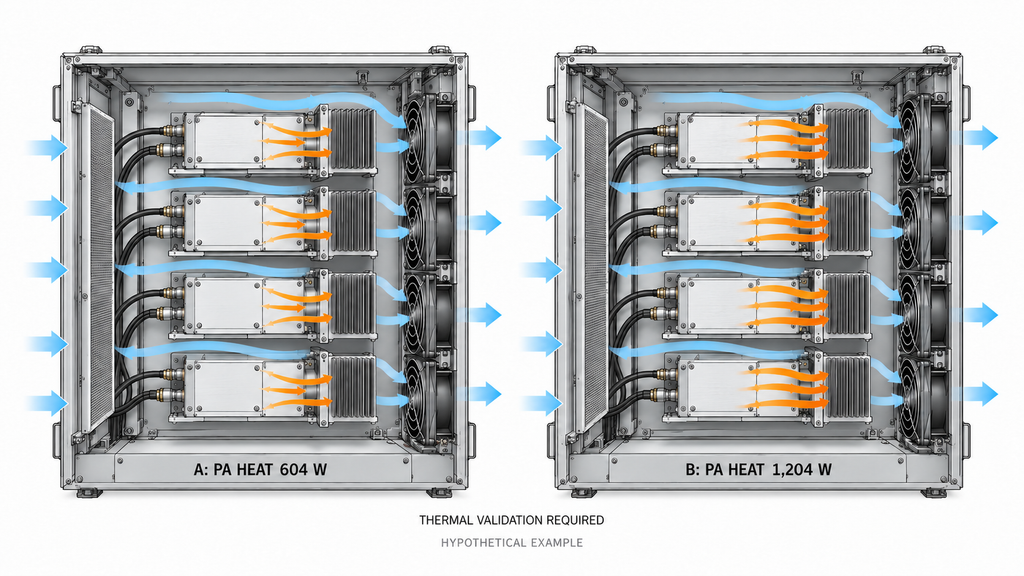
The approximate module heat balance is Pheat ≈ Pdc + Pin,net − Pout,net, with all terms referring to the same physical module boundary. It accounts for the RF drive energy entering the module; it must not then be counted again as a separate heat contribution. Additional supplies or external equipment require their own boundaries.
Illustrative four-module comparison. Assume both options deliver a net 100 W at each PA output reference plane, each takes 1 W of net RF drive, both have 28 V at the PA DC terminals, and four modules transmit simultaneously at the specified operating point. The 40% and 25% module efficiencies are hypothetical inputs—not RF SKYPOWER specifications or measured model results.
| Case | PA-port Pout / module | Module DC-to-RF efficiency | Net RF Pin / module | Vdc at PA | Pdc / module | Idc / module | Active modules | Total PA Pdc | Heat / module | Total PA heat |
|---|---|---|---|---|---|---|---|---|---|---|
| A: higher efficiency | 100 W | 40% | 1 W | 28 V | 250 W | 8.93 A | 4 | 1,000 W | 151 W | 604 W |
| B: lower efficiency | 100 W | 25% | 1 W | 28 V | 400 W | 14.29 A | 4 | 1,600 W | 301 W | 1,204 W |
| B minus A | 0 W | −15 percentage points | 0 W | 0 V | 150 W | 5.36 A | 0 | 600 W | 150 W | 600 W |
Swipe horizontally to compare all eleven fields →
At this simultaneous operating point, RF amplifier current consumption increases from 8.93 A to 14.29 A per module at 28 V. Across four simultaneously active modules, option B therefore draws 600 W more PA DC input and produces 600 W more PA heat. Neither number directly specifies a monetary saving or the change in cooling-equipment electricity. The heat-load calculation from amplifier efficiency establishes the thermal load; the installed configuration and supplier quotes determine its cost.
If fewer modules operate simultaneously, or the output and duty cycle change by operating state, the integrator must calculate those states separately rather than multiply a peak number across the entire system lifetime.
3. When Does PA Efficiency Change the 28 V Power Supply Budget?
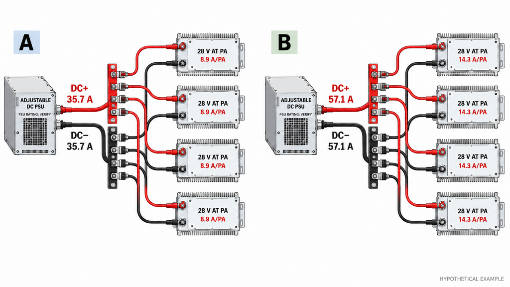
Lower PA DC demand reduces the power-supply load budget. The PSU purchase price changes only if that lower load changes a feasible, quoted configuration. In the four-module example, 1,000 W and 1,600 W correspond to approximately 35.7 A and 57.1 A at the specified 28 V PA terminals, before auxiliary equipment and distribution losses.
For each candidate, sum the loads that can operate at the same time, then add separately identified auxiliary loads. RF amplifier power supply requirements must be specified at the PA terminals, including operating voltage and continuous and transient current demand. The PSU engineer must then verify available output under the installation’s input voltage and ambient temperature, load-dependent derating, redundancy requirements, and cable, connector and protection-device losses. The voltage set at the PSU is not necessarily the voltage delivered at a high-current PA terminal. No universal percentage of “extra headroom” can substitute for the actual ratings and project constraints.
If both options fit the same required redundant PSU assembly, the 600 W difference produces no PSU purchase saving. If option B crosses a capacity, distribution or redundancy tier, its quoted PSU and wiring costs may rise. The mechanisms behind DC power-supply stress help identify design risks, but do not establish equipment prices.
The deliverable is two PSU configurations meeting identical environmental and availability requirements, each backed by a supplier rating curve, bill of materials and quote. Without those records, retain the DC difference but leave the capital-cost conclusion open.
4. How Do Higher Heat Loads Change Cooling and Cabinet Costs?
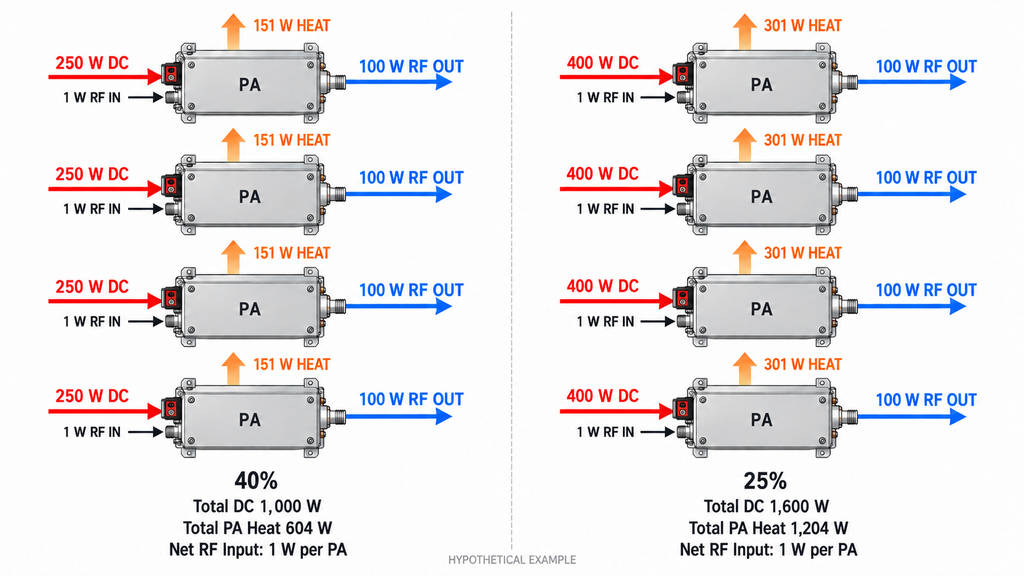
Heat-load figures become costs only after both options are shown to satisfy the same thermal and mechanical constraints. In the illustrative operating state, the cabinet designer would assess approximately 604 W of PA heat for option A and 1,204 W for option B, plus other heat sources within the chosen enclosure boundary. Neither figure directly determines the number of fans, cabinet volume, or electrical power consumed by cooling equipment.
The evaluation must keep the design ambient temperature, solar exposure where applicable, permitted component temperatures, air paths, enclosure sealing, noise limits, maintenance space and sustained operating condition consistent. An existing cabinet and cooling assembly may accommodate either option with acceptable margin; in that case, higher efficiency improves thermal margin without necessarily reducing the purchase bill. A different project may require a larger enclosure, more capable fans, a different cold plate or another heat-rejection arrangement for option B.
Each option needs a validated cooling and cabinet configuration with a comparable quote, including space and service access. The RF power amplifier thermal management checks help establish whether each cooling design can meet its operating limits; comparable supplier quotes are still needed to determine cost. Check whether PA efficiency affects the required cabinet size before claiming an enclosure saving. Until both designs pass the defined hot-state requirements, the calculated heat-load difference is the only established result.
5. How Should Energy Use and Maintenance Enter Five-Year TCO?
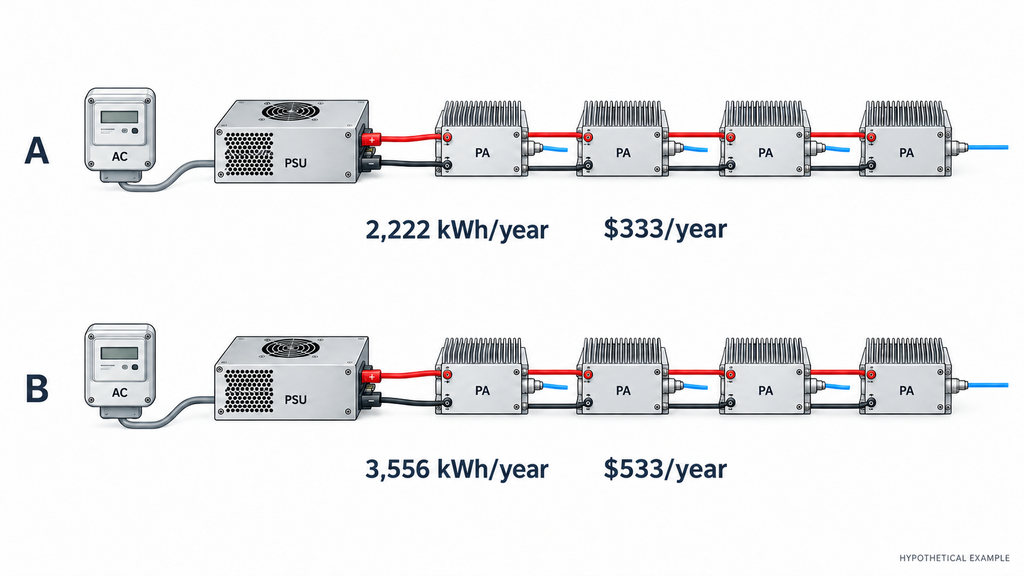
Annual electricity cost depends on operating-state hours, PSU efficiency at each load and the tariff. For each RF-on state, estimate AC energy at the PSU input from its total DC output load and efficiency at that load:
E_AC,on,year (kWh) = Σ over RF-on states s {[(P_PA,term,s + P_dist,s + P_aux,s) / η_PSU,s] × (h_s / 1,000)}
Here, P_PA,term,s is the aggregate PA load measured at the module DC terminals, P_dist,s is wiring and distribution loss between the PSU and those terminals (which can increase with current), and P_aux,s covers other loads powered by that PSU but not already counted. Each h_s is annual hours in that RF-on state, and η_PSU,s must correspond to the total PSU output load. All power terms are in watts. For standby or off states, use measured AC input or a documented no-load/standby rating and actual hours rather than extrapolating an RF-on efficiency value down to zero load.
Apply the electricity tariff to all included states. Count loads on other supplies within a consistent boundary, and calculate cooling-equipment electricity from its electrical demand and hours. If a metered PSU AC figure already includes distribution and auxiliary loads, do not add them again. Waste-heat watts are not a second electrical load.
For a PA-only extension of the hypothetical four-module case, omit distribution and auxiliary terms. Assume both PSUs are 90% efficient at their respective RF-on load points, all four PAs run at that point for 2,000 equivalent hours per year, and electricity costs $0.15/kWh. Option A’s PA-related AC input is about 1.111 kW and option B’s about 1.778 kW. This gives approximately 2,222 versus 3,556 kWh, or $333 versus $533 per year: about $200 annually and $1,000 over five undiscounted years. These are hypothetical figures, not measured product savings. Distribution losses, standby and off-state energy, cooling electricity, other loads, equipment and maintenance are excluded and need their own project inputs.
Maintenance belongs in the model when there are comparable service quotations or project records for fans, filters, spares, inspection, repair or replacement. Lower heat may affect maintenance, but it does not establish a numerical failure-rate reduction. Where service evidence is absent, mark the cost as unpriced rather than inventing an annual saving. Short seasonal missions and high-duty installations can produce very different purchasing decisions even with the same instantaneous 600 W DC difference.
6. Which PA Option Has the Lower Total Cost of Ownership?
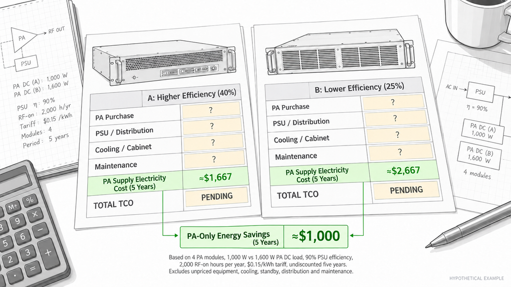
Rank the options by five-year project TCO only after they meet identical RF, thermal and availability conditions and their quoted costs cover the same scope. Comparing amplifier purchase prices before pricing the associated PSU, cooling and cabinet configuration can reverse the shortlist for the wrong reason.
Build a Five-Year TCO Comparison
Use one currency, one five-year horizon and equivalent installed functions, with the same present-value method for both options or an explicitly undiscounted total. Add amplifier acquisition, power and distribution hardware, cooling, enclosure, relevant installation and acceptance, electricity and supported maintenance. The illustration and threshold below exclude unpriced replacement, downtime and residual value. A real project may add evidenced replacement or downtime costs and residual-value credits on the same accounting and discounting basis, without duplicating an existing line.
The table compares hypothetical option A (40% module efficiency) with option B (25%). Only the PA-supply electricity row has a numerical illustration; every other cost needs a matched quotation or project record.
| Cost item | Option A: higher efficiency | Option B: lower efficiency | Calculation or quotation basis | Input status |
|---|---|---|---|---|
| PA modules, one-time | Comparable supplier quote required | Comparable supplier quote required | Same module count and RF specification | Unpriced |
| PSU and DC distribution, one-time | Rated configuration quote required | Rated configuration quote required | Continuous load, derating, redundancy and harness scope | Unpriced |
| Cooling hardware, one-time | Thermal-design quote required | Thermal-design quote required | Same ambient and heat-rejection constraints | Unpriced |
| Cabinet and mechanical integration, one-time | Enclosure quote required | Enclosure quote required | Same ingress, space and service requirements | Unpriced |
| Installation and acceptance, where in scope | Project quote required | Project quote required | Same labor and verification boundary | Unpriced |
| PSU AC electricity during RF-on states, per year | About $333/year | About $533/year | PA-only illustration: 2,000 h, 90% PSU efficiency, $0.15/kWh; full PSU load unpriced | Hypothetical only |
| Standby and off-state AC electricity per year | Measured or vendor-rated input required | Measured or vendor-rated input required | Actual idle/off power and hours; no RF-on efficiency extrapolation | Unpriced |
| Additional cooling electricity per year | Measured or vendor-model input required | Measured or vendor-model input required | Cooling electrical demand and actual hours | Unpriced |
| Maintenance and service per year | Comparable service input required | Comparable service input required | Maintenance scope and available records | Unpriced |
| Replacement or downtime, only if substantiated | Excluded from illustration; include only if evidenced | Excluded from illustration; include only if evidenced | Do not duplicate warranty or maintenance costs | Conditional |
| Five-year TCO | CapEx(A) + PV(OpEx(A), years 1–5) | CapEx(B) + PV(OpEx(B), years 1–5) | Or consistently use undiscounted five-year OpEx sums | Not rankable yet |
| Five-year cost difference | Not yet calculable | Not yet calculable | TCO(B) − TCO(A); a positive result favors A | Depends on missing inputs |
| Break-even PA price premium | Maximum extra price supported by other savings | Lower-efficiency price baseline | Apply the threshold formula below | Not determined by energy alone |
Swipe horizontally to review the complete five-year cost basis →
An integrator should keep the one-time quotes separate from annual costs and identify which items are included in bundled supplier prices. For example, a fan included in a cabinet quote should not appear again as separately purchased cooling hardware. The value of five years is a comparison horizon here, not a claimed product service life.
Calculate the Break-Even Price Premium
Let H represent the higher-efficiency option and L the lower-efficiency baseline. The maximum additional PA purchase price justified by other savings is:
ΔC_PA,max = (Other CapEx_L − Other CapEx_H) + [PV(OpEx_L) − PV(OpEx_H)]
Here, “other CapEx” includes the quoted PSU, distribution, cooling, cabinet and relevant installation differences, excluding PA purchase price. Operating expenditure includes documented electricity, cooling electricity and maintenance over the same horizon. In this illustration, no unpriced replacement, downtime or residual-value term enters the threshold. If present-value discounting is not used, replace PV with consistently undiscounted five-year sums and state that choice. Count each cost once.
If PA purchase price_H − PA purchase price_L ≤ ΔC_PA,max, the higher-efficiency premium is recovered within the modeled costs and assumptions. Above that threshold, option L has the lower modeled TCO, provided both remain technically acceptable. The threshold can be zero or negative.
For the PA-only example, suppose non-PA capital costs are identical and all other operating costs are equal or excluded for both options: distribution losses, auxiliary loads, standby/off-state electricity, cooling electricity and maintenance. The undiscounted five-year PA-supply energy advantage is then $1,000. This is the maximum PA purchase premium supported by that single modeled saving, not an RF SKYPOWER price or a full-project TCO result.
Fewer RF-on hours or lower tariffs reduce the energy advantage; more hours or higher tariffs increase it. When both options fit the same PSU and cooling hardware tiers, enter no capital saving for those items. A change in PSU, cooling or cabinet tier affects the premium only when supported by comparable equipment quotes. Calculate each PSU’s efficiency at its own load point, and keep the purchasing decision open until material costs are documented.
What Should a C-UAS RFQ Include for a Defensible Cost Comparison?
A defensible RFQ gives every supplier the same RF duty and delivery boundary. The integrator should define the frequency range, net PA-output power and reference plane, waveform and duty cycle, simultaneously active modules, 28 V terminal requirements, load and installation conditions, maximum design ambient, expected operating-state hours and the cost-evaluation period. It should also specify which PSU, distribution, cooling, cabinet, acceptance, maintenance and warranty items the supplier must include or exclude.
The PA supplier should identify the exact model and revision and provide efficiency definitions, RF drive/output conditions, DC current or power across the relevant states, and thermal data with the supporting evidence. PSU and cooling vendors quote configurations meeting the same environmental and redundancy limits. The project owner supplies the tariff and realistic operating hours. Procurement records currency, tax and delivery scope, lead time, quotation validity, warranty and service boundaries. Label every TCO input as measured, quoted, assumed or pending in the comparison sheet. If material inputs remain pending, the table is not yet a ranked bid result. This keeps RF PA quotations before shortlisting technically comparable while the TCO model evaluates project cost.
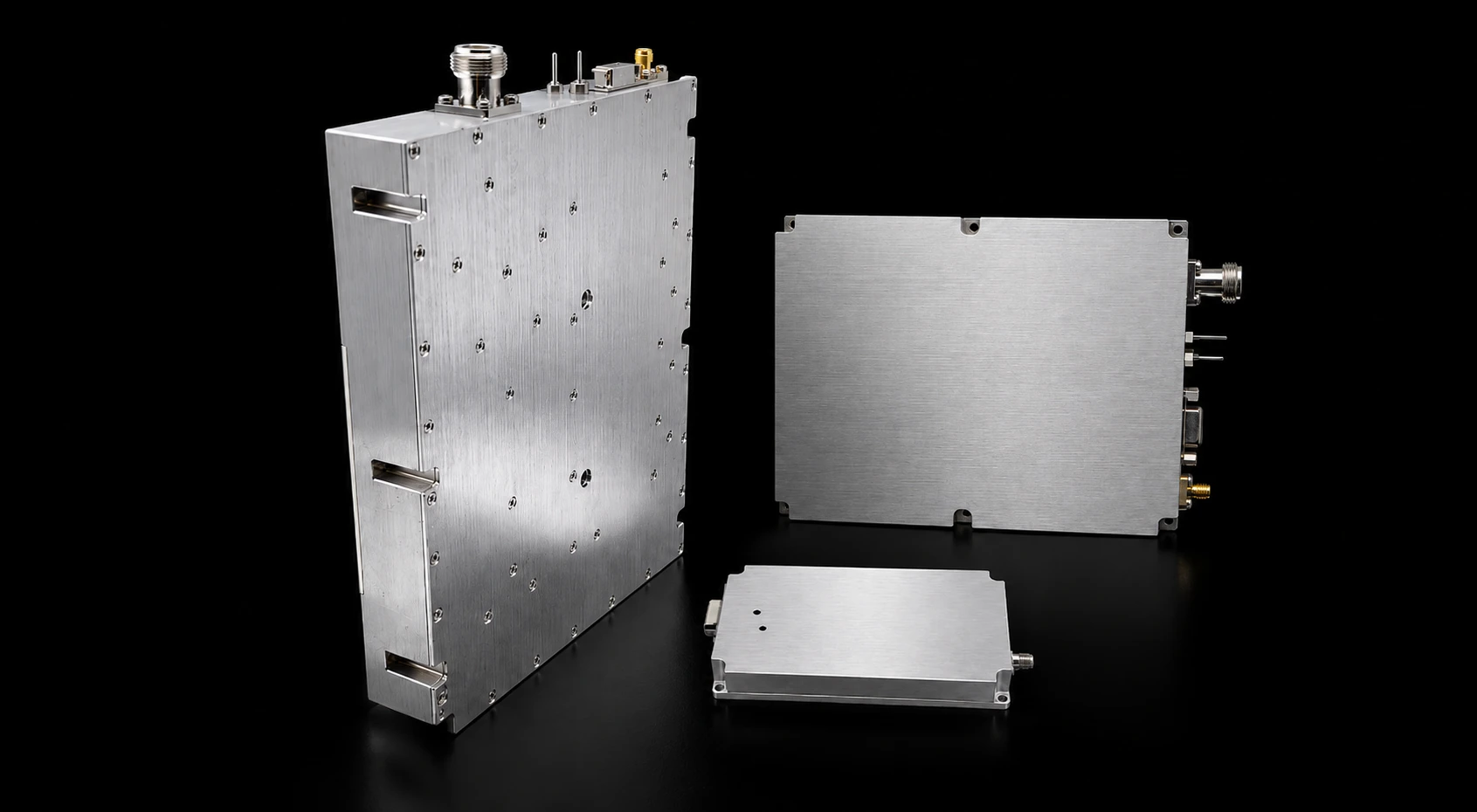
Use the RF SKYPOWER RF power amplifier module range to identify candidates, then request efficiency and thermal evidence for the exact model and revision. A product-range page cannot establish an individual model’s efficiency or five-year cost.
Wideband RF PA Modules
Select a frequency band to compare standard 30 W–200 W models and open the applicable English PDF datasheets.
30–512 MHz · 5 standard models
| Power | Model / PDF | Psat min. / typ. | Current typ. / max. | Dimensions | RF input / output | Control |
|---|---|---|---|---|---|---|
| 30 W | 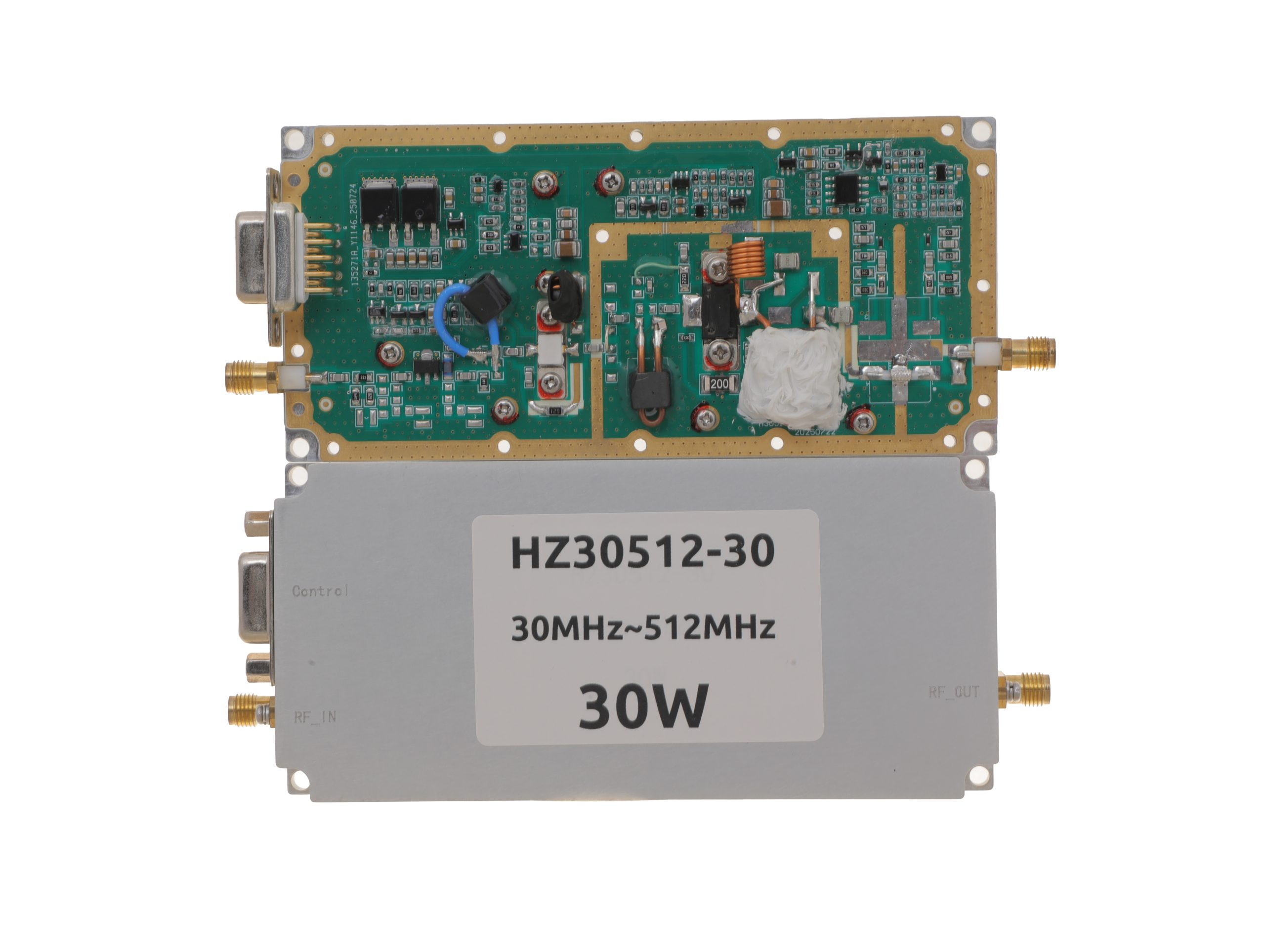 HZ30512-30NA1Open English PDF ↗ | 25 / 30 W | 3.2 / 4 A | 125 × 59 × 21.5 mmWeight: 0.5 kg | SMA-KFD46 / SMA-KFD46 | 9-pin D-Sub |
| 50 W | 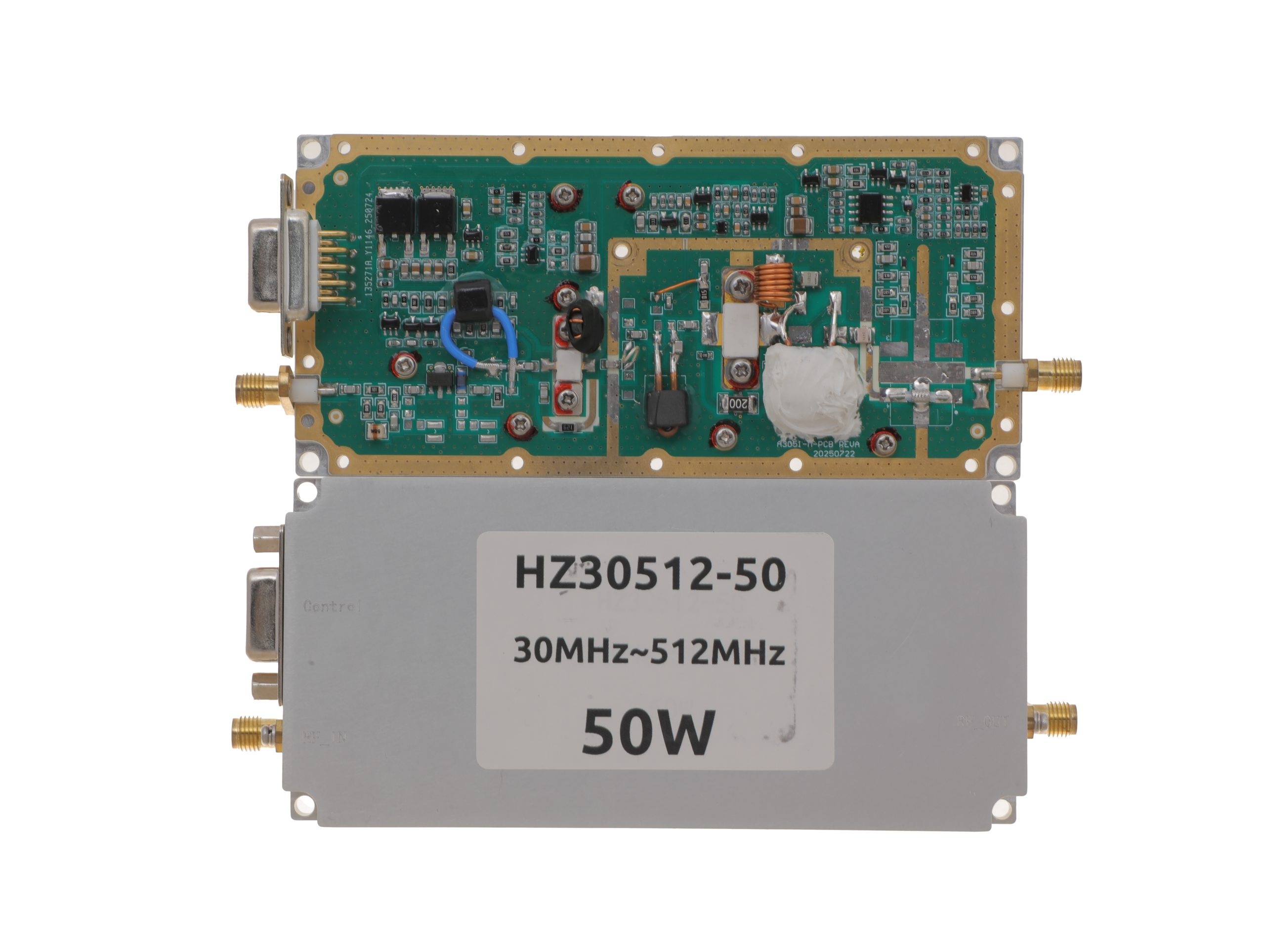 HZ30512-50NA1Open English PDF ↗ | 40 / 50 W | 7.2 / 9 A | 125 × 59 × 21.5 mmWeight: 0.5 kg | SMA-KFD46 / SMA-KFD46 | 9-pin D-Sub |
| 100 W | 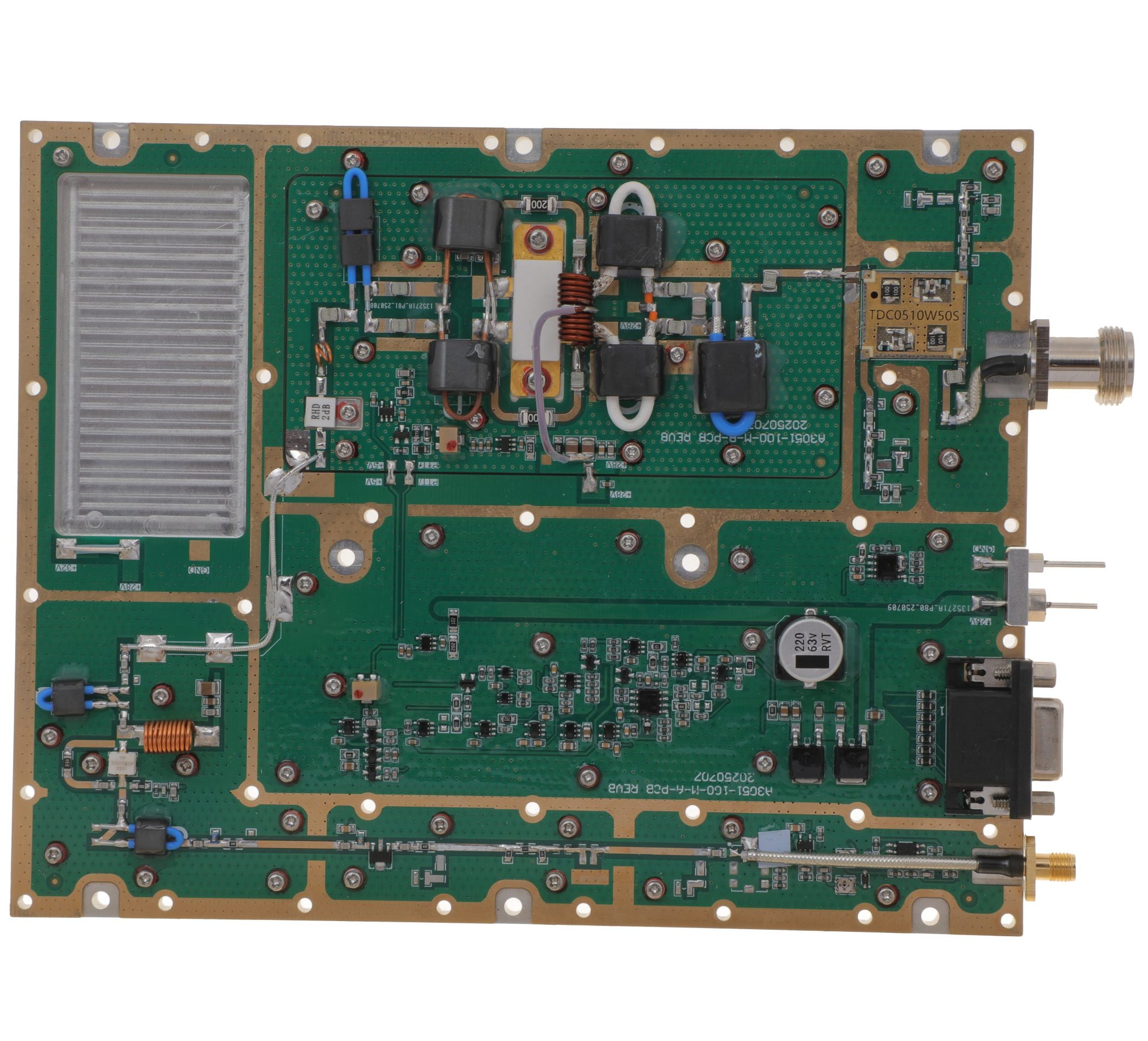 HZ30512-100NA1Open English PDF ↗ | 80 / 100 W | 14.5 / 18 A | 160 × 120 × 25 mmWeight: 1.4 kg | SMA-F / N-F | 15-pin D-Sub |
| 150 W | 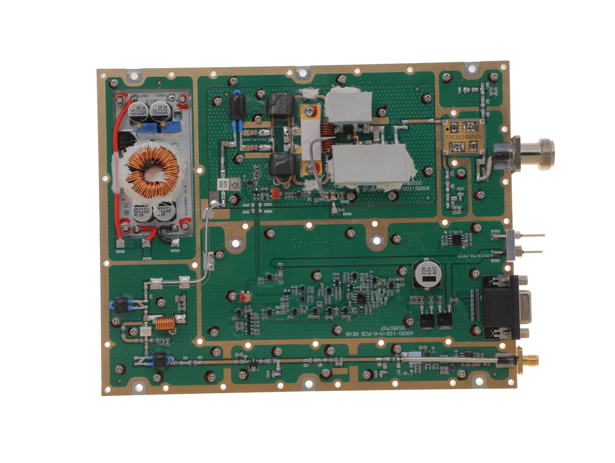 HZ30512-150NA1Open English PDF ↗ | 120 / 150 W | 16 / 20 A | 200 × 158 × 25 mmWeight: 1.4 kg | SMA-F / N-F | 15-pin D-Sub |
| 200 W | 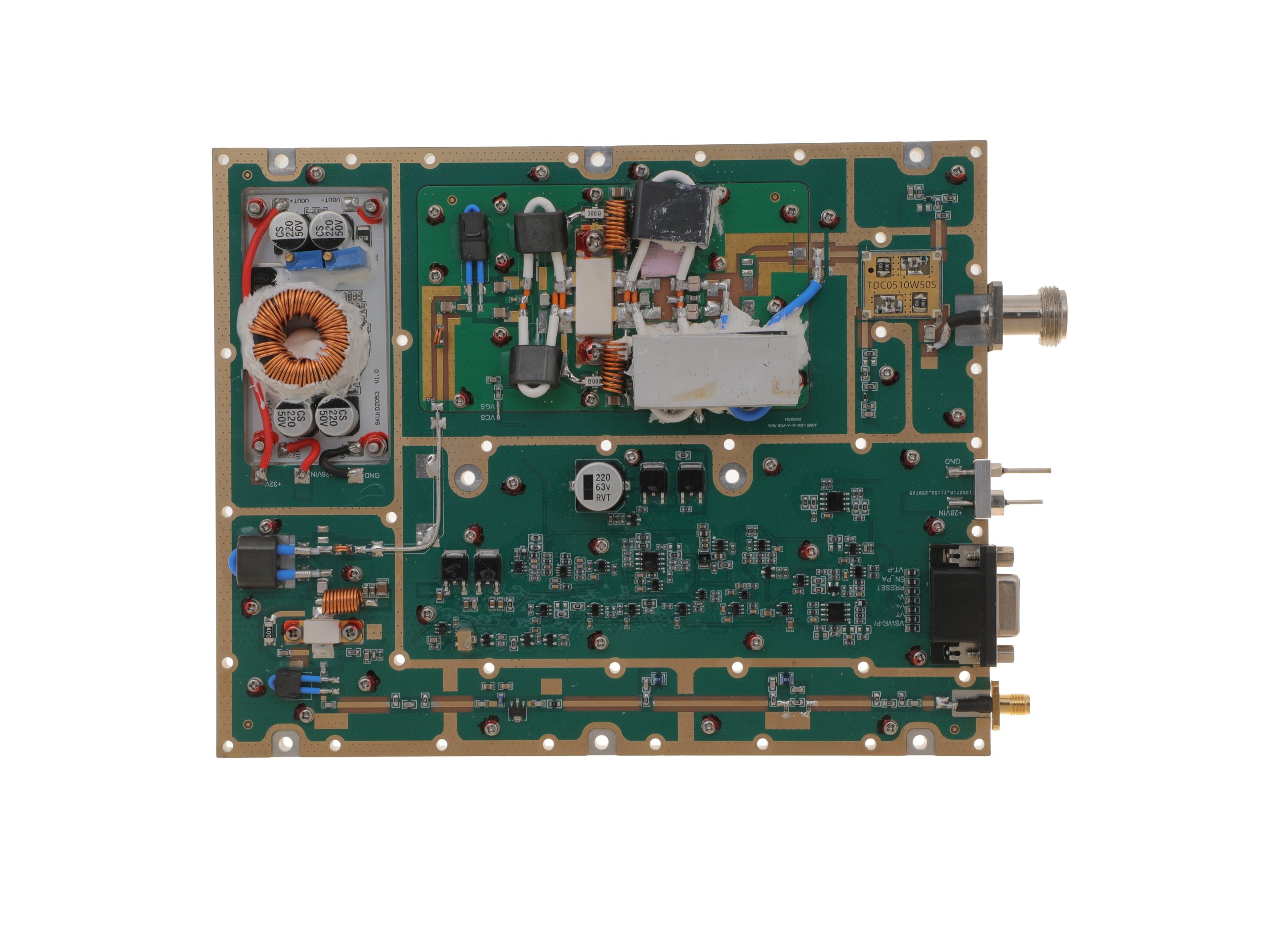 HZ30512-200NA1Open English PDF ↗ | 160 / 200 W | 29 / 36 A | 200 × 158 × 25 mmWeight: 1.4 kg | SMA-F / N-F | 15-pin D-Sub |
300–1200 MHz · 5 standard models
| Power | Model / PDF | Psat min. / typ. | Current typ. / max. | Dimensions | RF input / output | Control |
|---|---|---|---|---|---|---|
| 30 W | 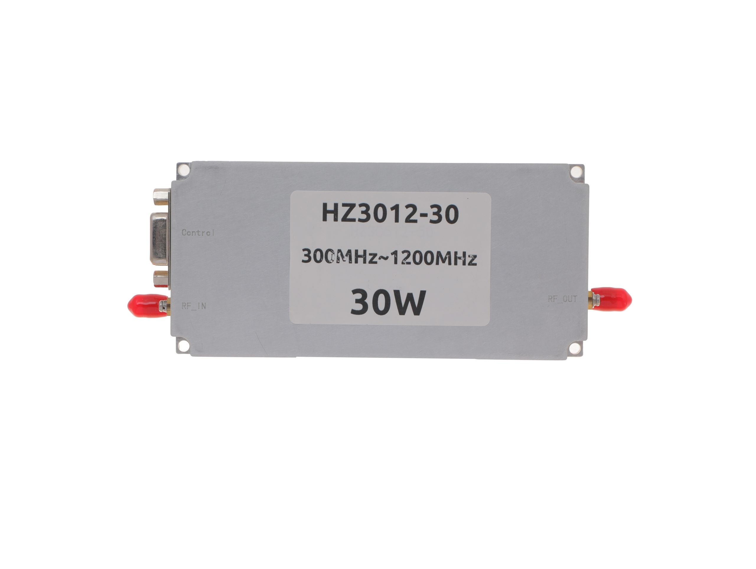 HZ3001200-30Open English PDF ↗ | 25 / 30 W | 2.4 / 3 A | 125 × 59 × 21.5 mm | SMA-KFD46 / SMA-KFD46 | 9-pin D-Sub |
| 50 W | 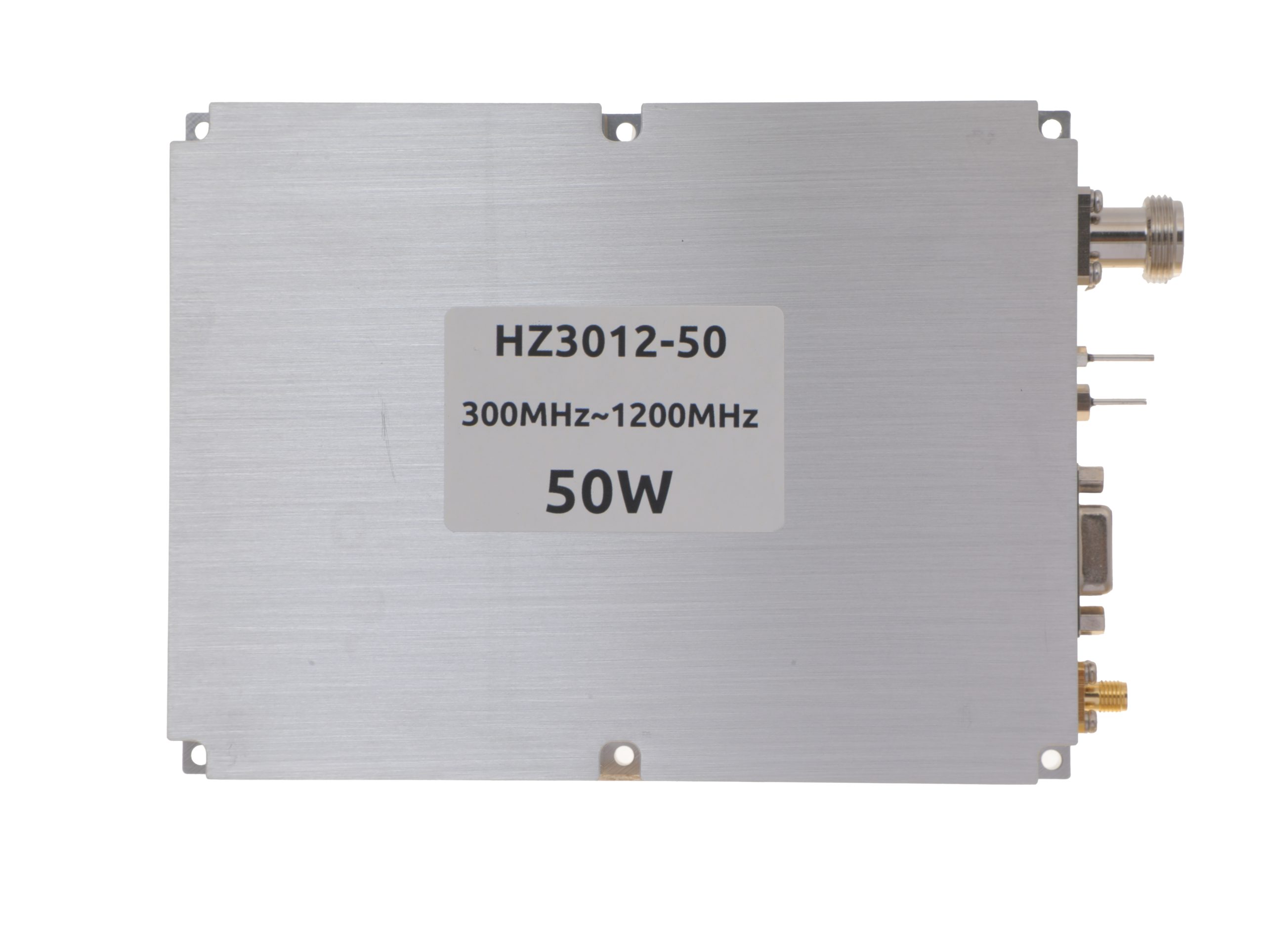 HZ3001200-50Open English PDF ↗ | 40 / 50 W | 5.6 / 7 A | 125 × 59 × 21.5 mm | SMA-KFD46 / SMA-KFD46 | 9-pin D-Sub |
| 100 W | 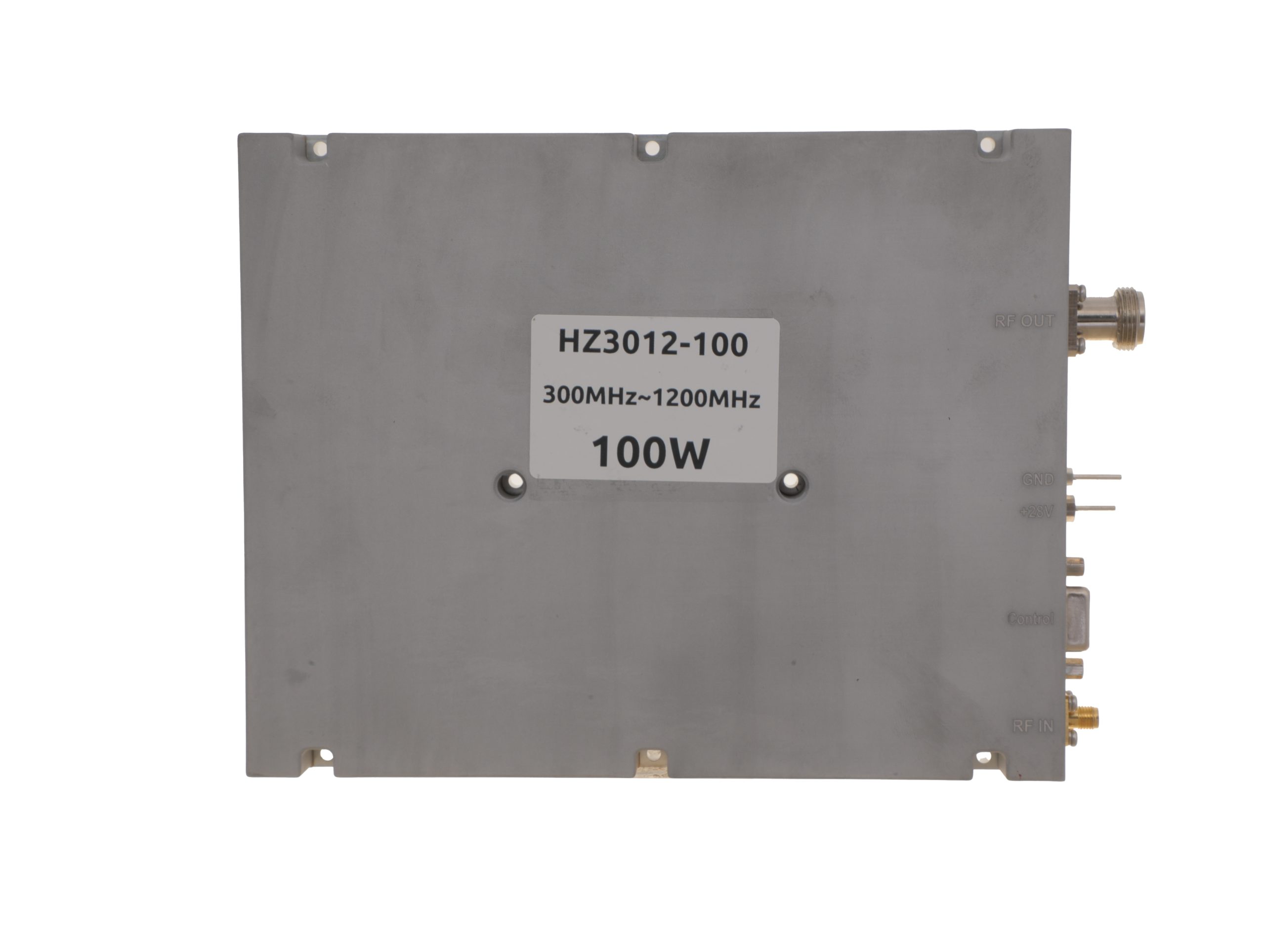 HZ3001200-100Open English PDF ↗ | 80 / 100 W | 11.5 / 14 A | 200 × 158 × 25 mm | SMA-F / N-F | 15-pin D-Sub |
| 150 W | 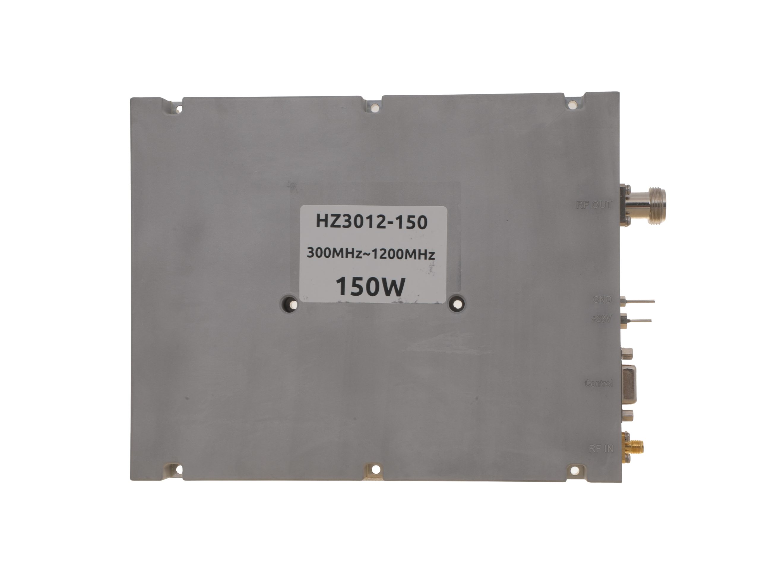 HZ3001200-150Open English PDF ↗ | 120 / 150 W | 18 / 22 A | 200 × 158 × 25 mm | SMA-F / N-F | 15-pin D-Sub |
| 200 W | 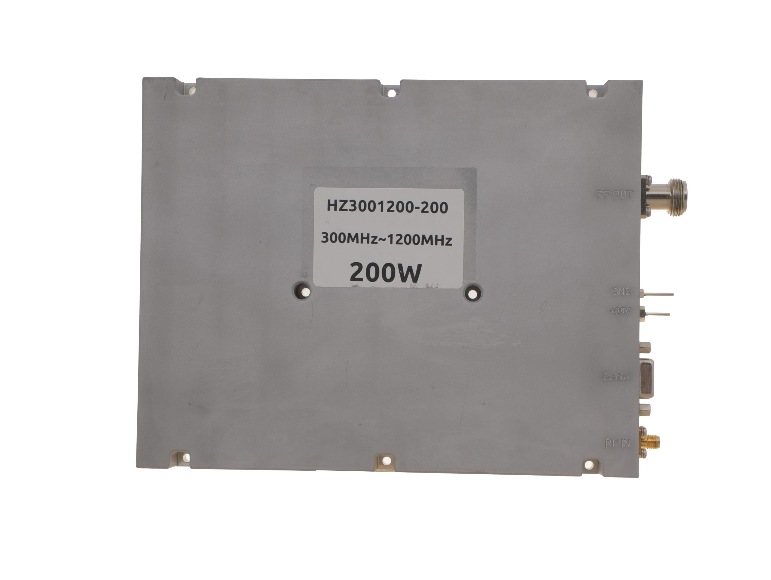 HZ3001200-200Open English PDF ↗ | 160 / 200 W | 24 / 29 A | 200 × 158 × 25 mm | SMA-F / N-F | 15-pin D-Sub |
300–1700 MHz · 5 standard models
| Power | Model / PDF | Psat min. / typ. | Current typ. / max. | Dimensions | RF input / output | Control |
|---|---|---|---|---|---|---|
| 30 W | 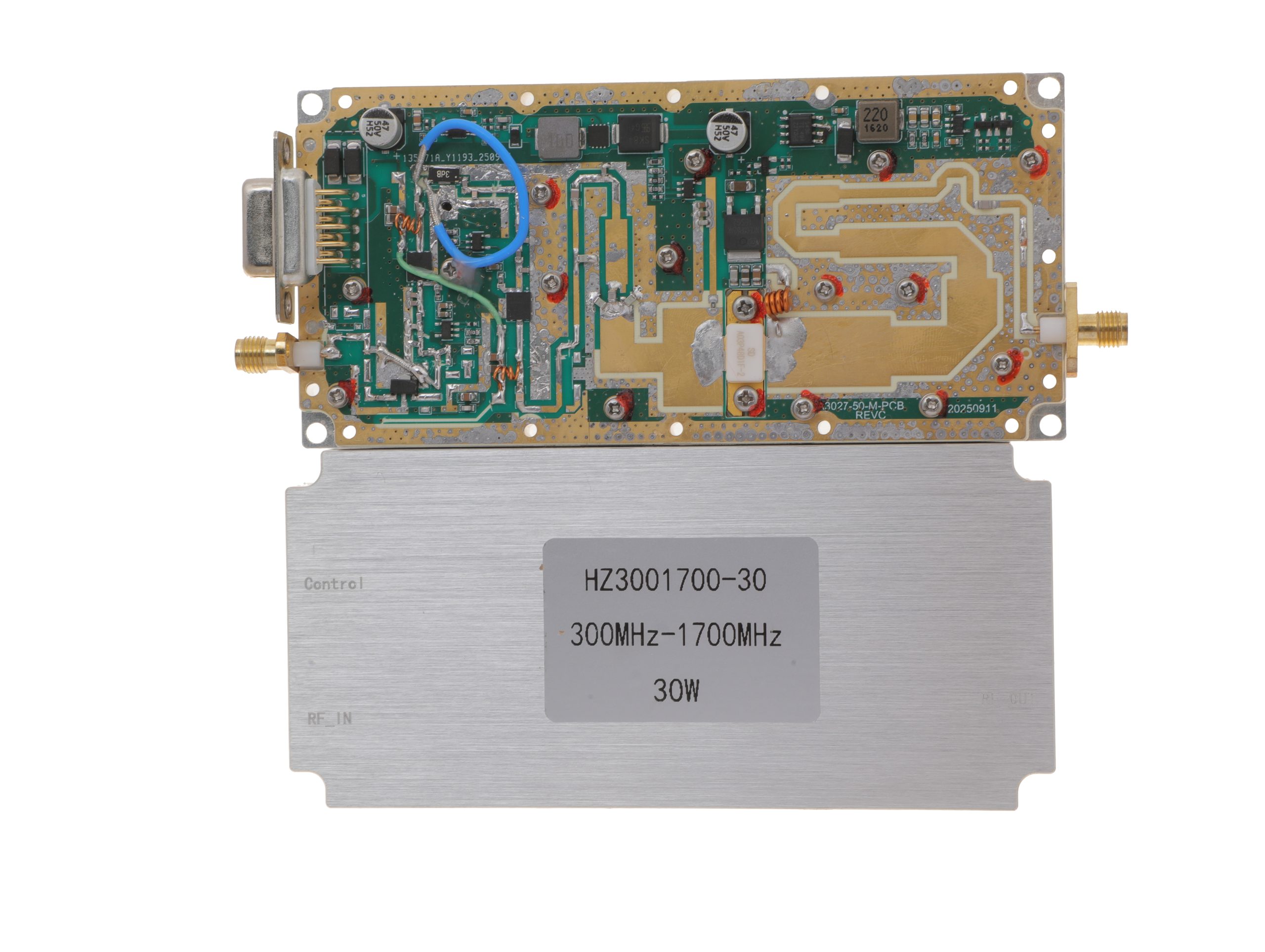 HZ3001700-30Open English PDF ↗ | 25 / 30 W | 2.4 / 3 A | 125 × 59 × 21.5 mm | SMA-KFD46 / SMA-KFD46 | 9-pin D-Sub |
| 50 W | 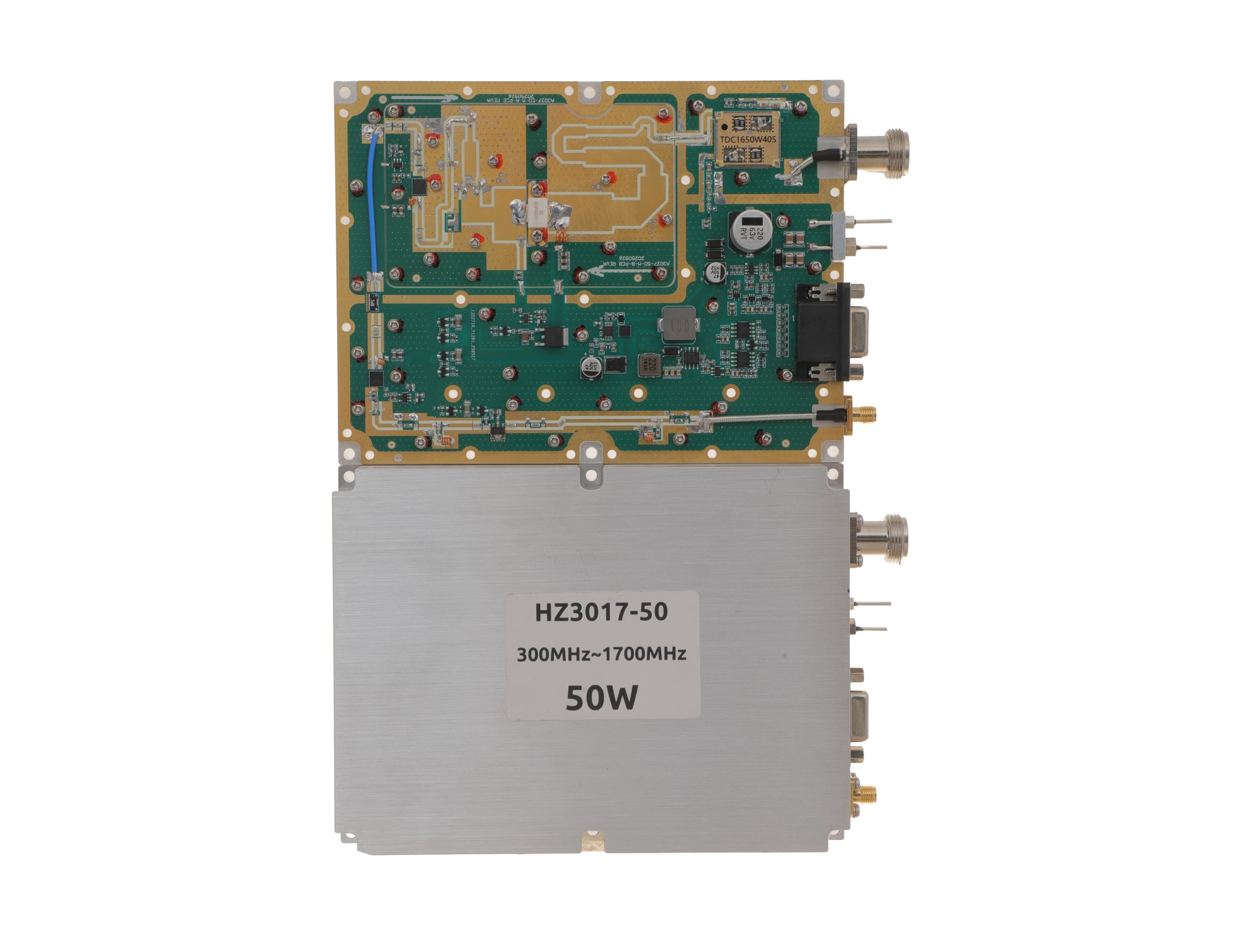 HZ3001700-50Open English PDF ↗ | 40 / 50 W | 5.6 / 7 A | 160 × 120 × 25 mm | SMA-F / N-F | 15-pin D-Sub |
| 100 W | 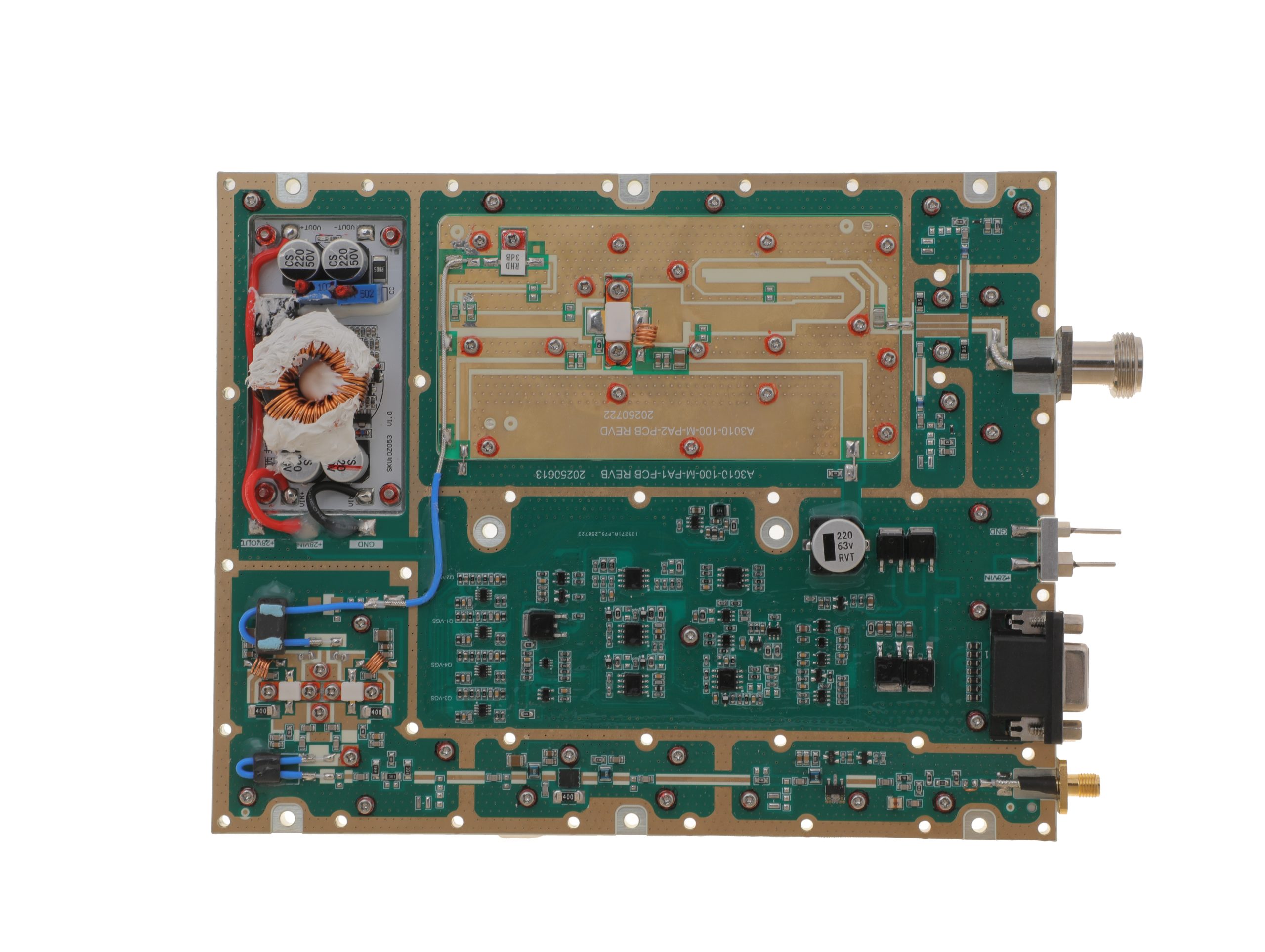 HZ3001700-100Open English PDF ↗ | 80 / 100 W | 11.5 / 14 A | 200 × 158 × 25 mm | SMA-F / N-F | 15-pin D-Sub |
| 150 W | 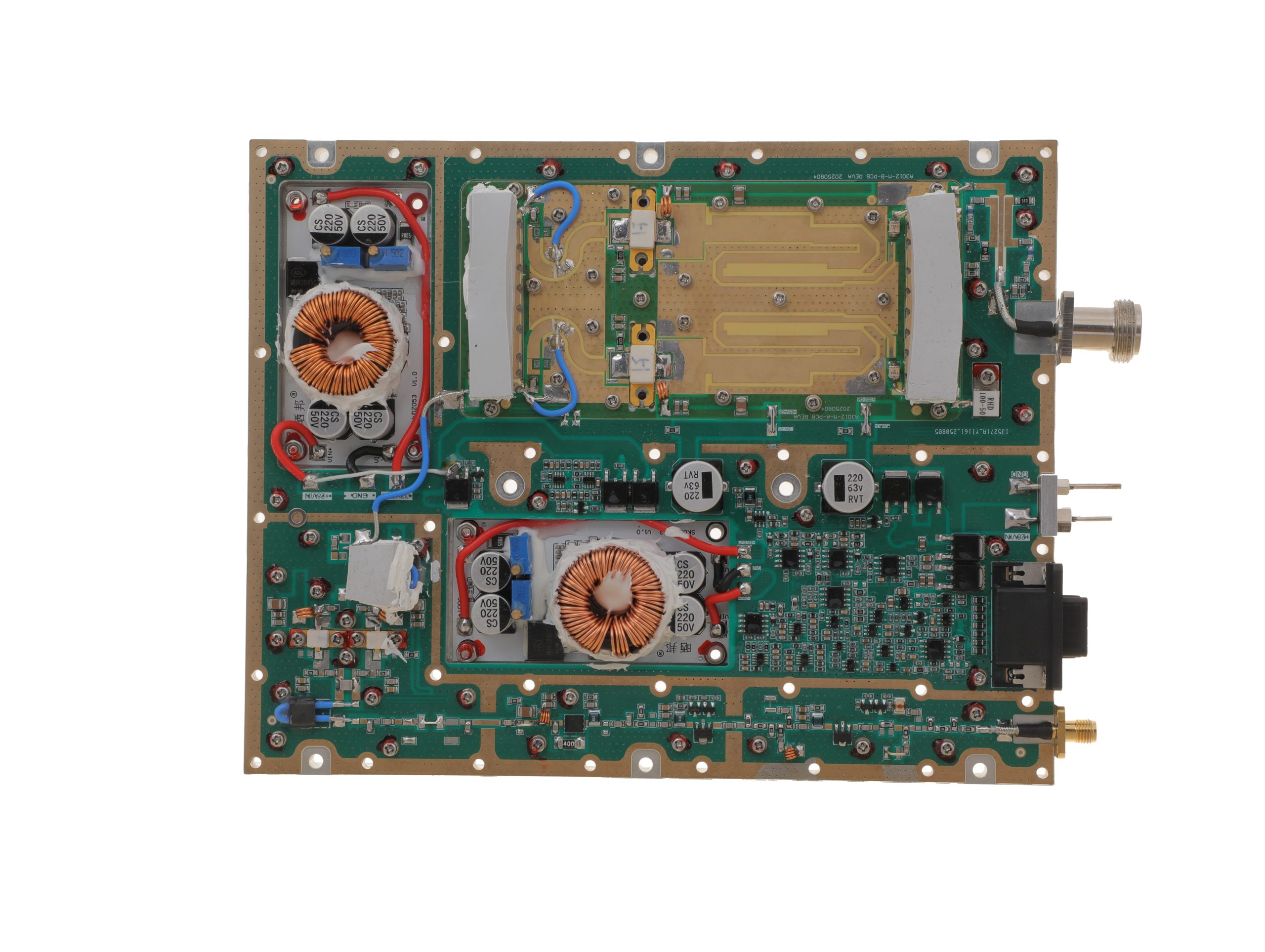 HZ3001700-150Open English PDF ↗ | 120 / 150 W | 18 / 22 A | 200 × 158 × 25 mm | SMA-F / N-F | 15-pin D-Sub |
| 200 W | 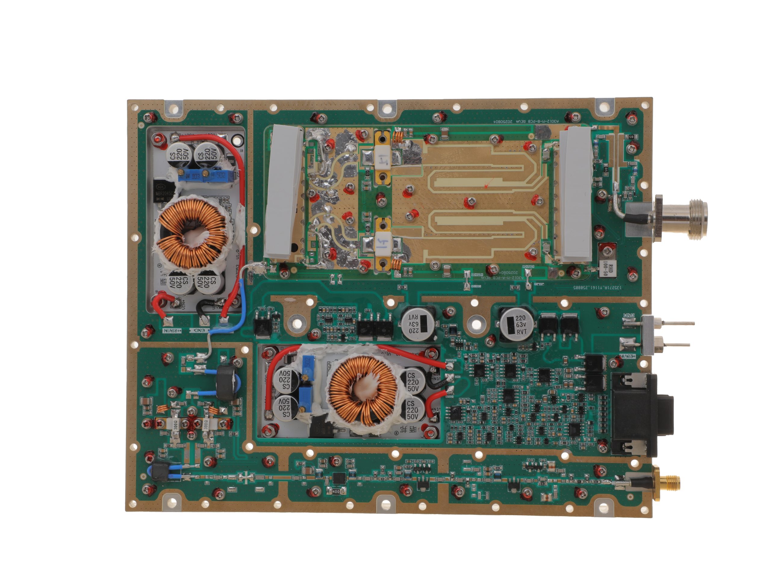 HZ3001700-200Open English PDF ↗ | 158 / 200 W | 24 / 29 A | 200 × 158 × 25 mm | SMA-F / N-F | 15-pin D-Sub |
300–2700 MHz · 5 standard models
| Power | Model / PDF | Psat min. / typ. | Current typ. / max. | Dimensions | RF input / output | Control |
|---|---|---|---|---|---|---|
| 30 W | 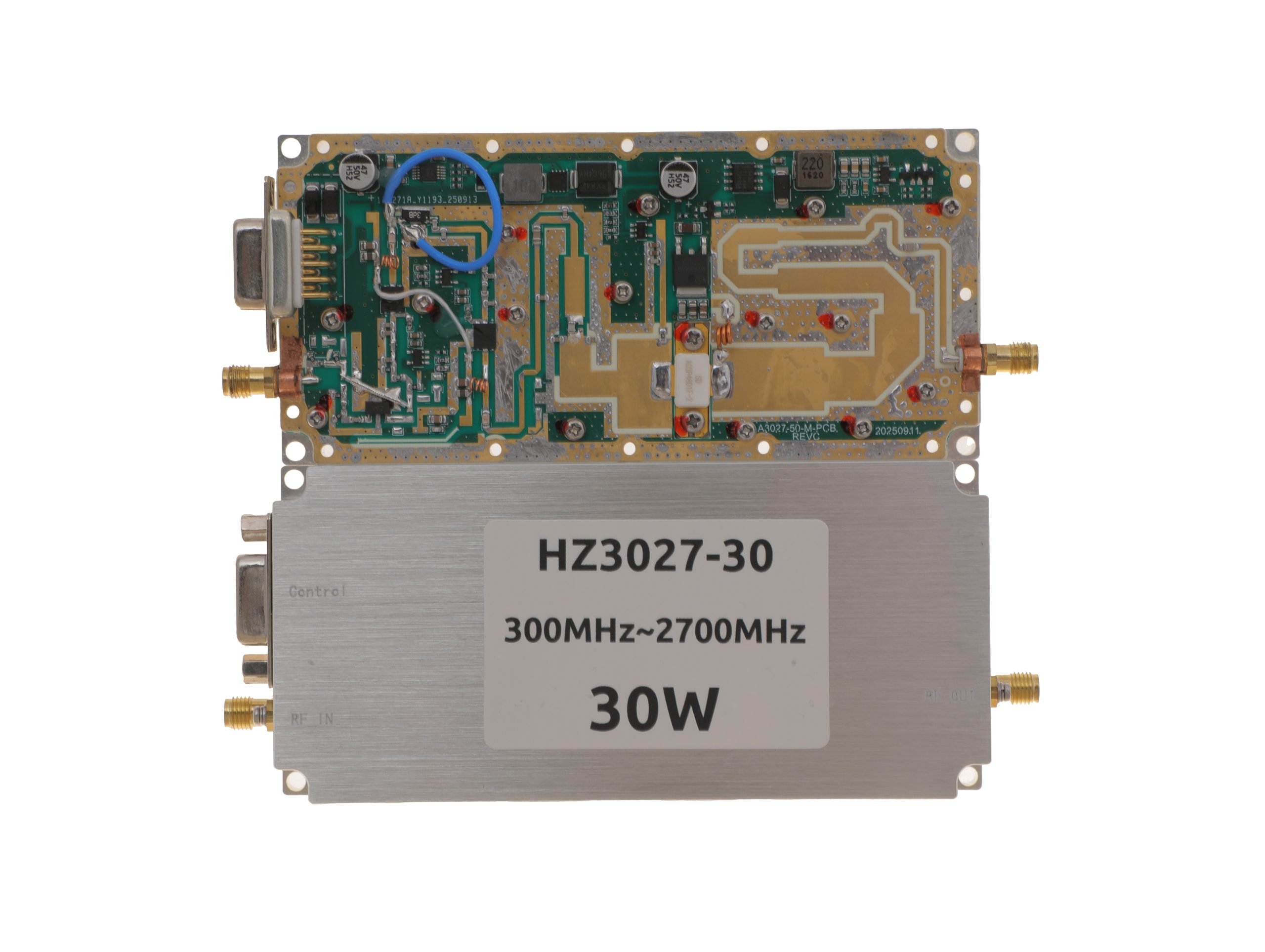 HZ3002700-30NA1Open English PDF ↗ | 25 / 30 W | 3.2 / 4 A | 125 × 59 × 21.5 mm | SMA-KFD46 / SMA-KFD46 | 9-pin D-Sub |
| 50 W | 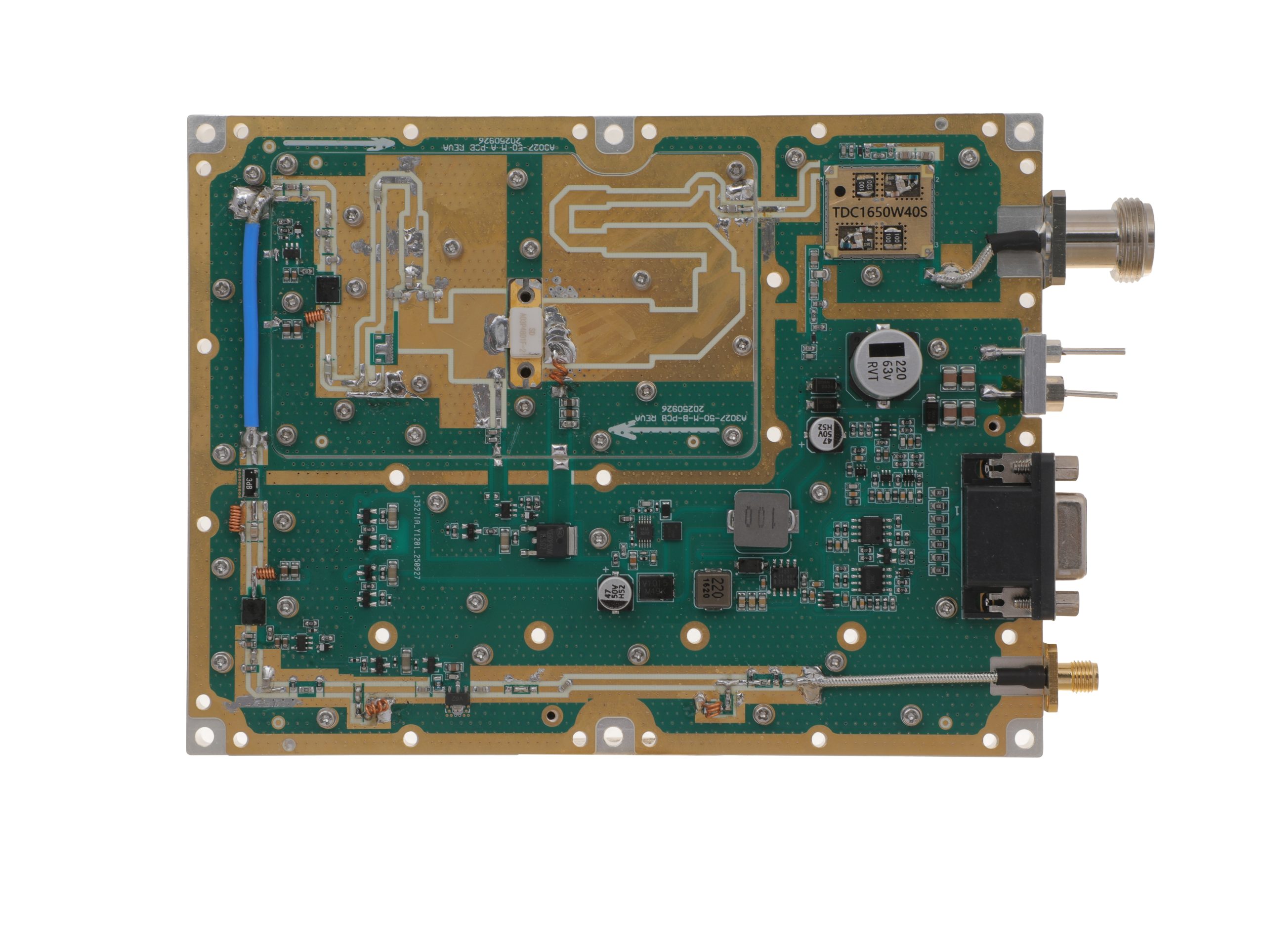 HZ3002700-50NA1Open English PDF ↗ | 40 / 50 W | 7.2 / 9 A | 160 × 120 × 25 mm | SMA-F / N-F | 15-pin D-Sub |
| 100 W | 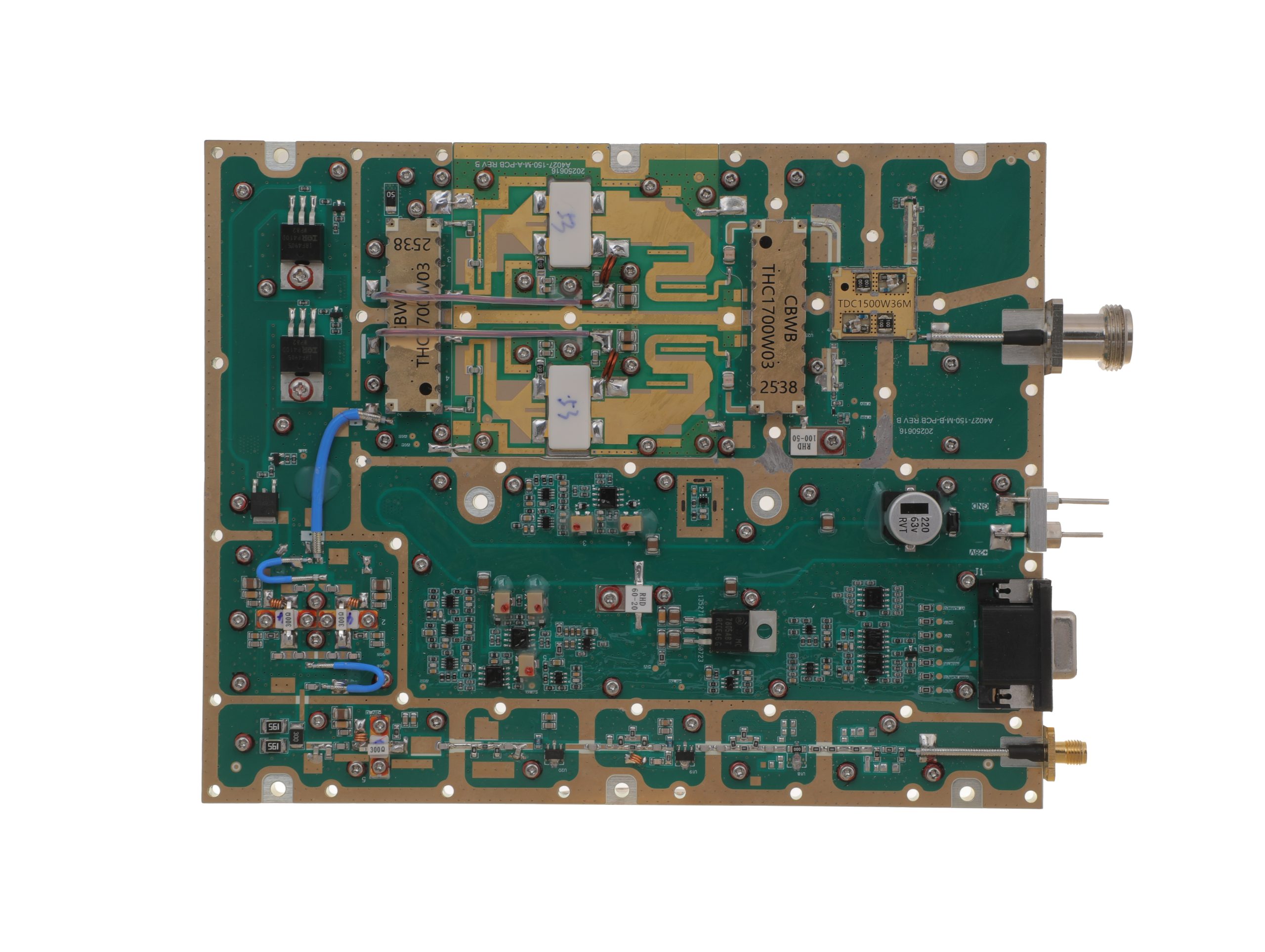 HZ3002700-100NA1Open English PDF ↗ | 80 / 100 W | 14.5 / 18 A | 200 × 158 × 25 mm | SMA-F / N-F | 15-pin D-Sub |
| 150 W | 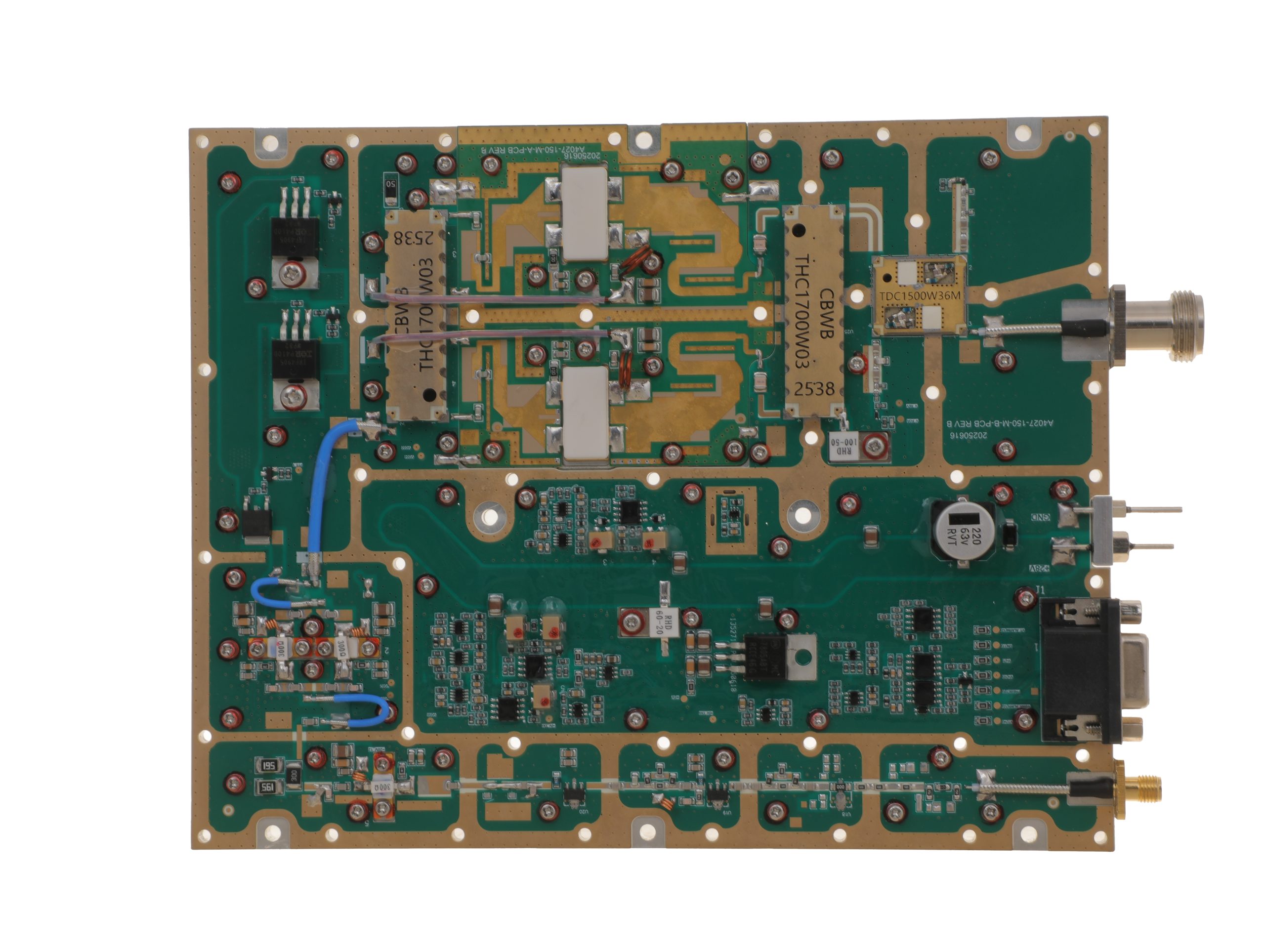 HZ3002700-150NA1Open English PDF ↗ | 120 / 150 W | 16 / 20 A | 200 × 158 × 25 mm | SMA-F / N-F | 15-pin D-Sub |
| 200 W | 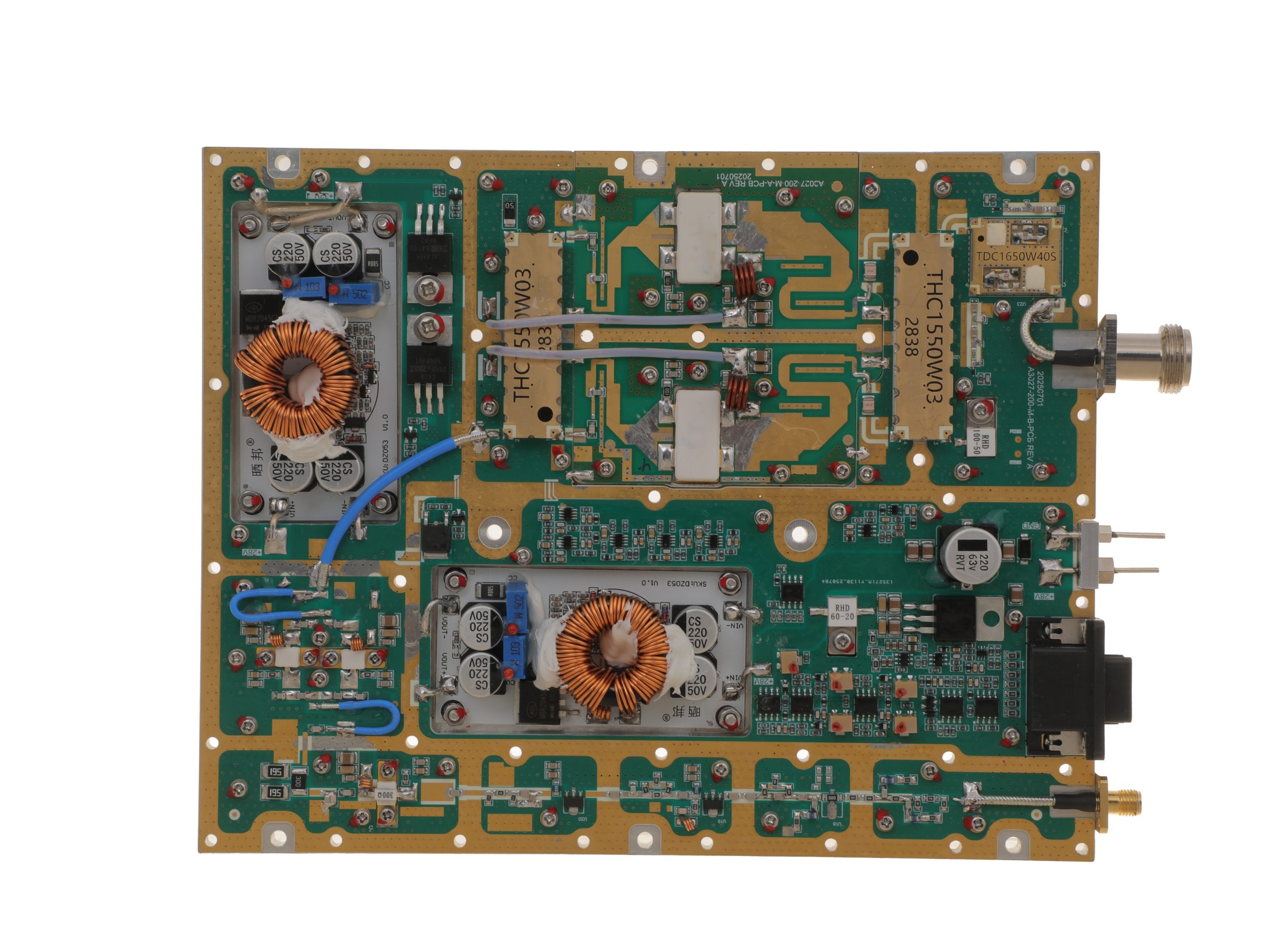 HZ3002700-200NA1Open English PDF ↗ | 160 / 200 W | 29 / 36 A | 200 × 158 × 25 mm | SMA-F / N-F | 15-pin D-Sub |
2000–6000 MHz · 5 standard models
| Power | Model / PDF | Psat min. / typ. | Current typ. / max. | Dimensions | RF input / output | Control |
|---|---|---|---|---|---|---|
| 30 W | 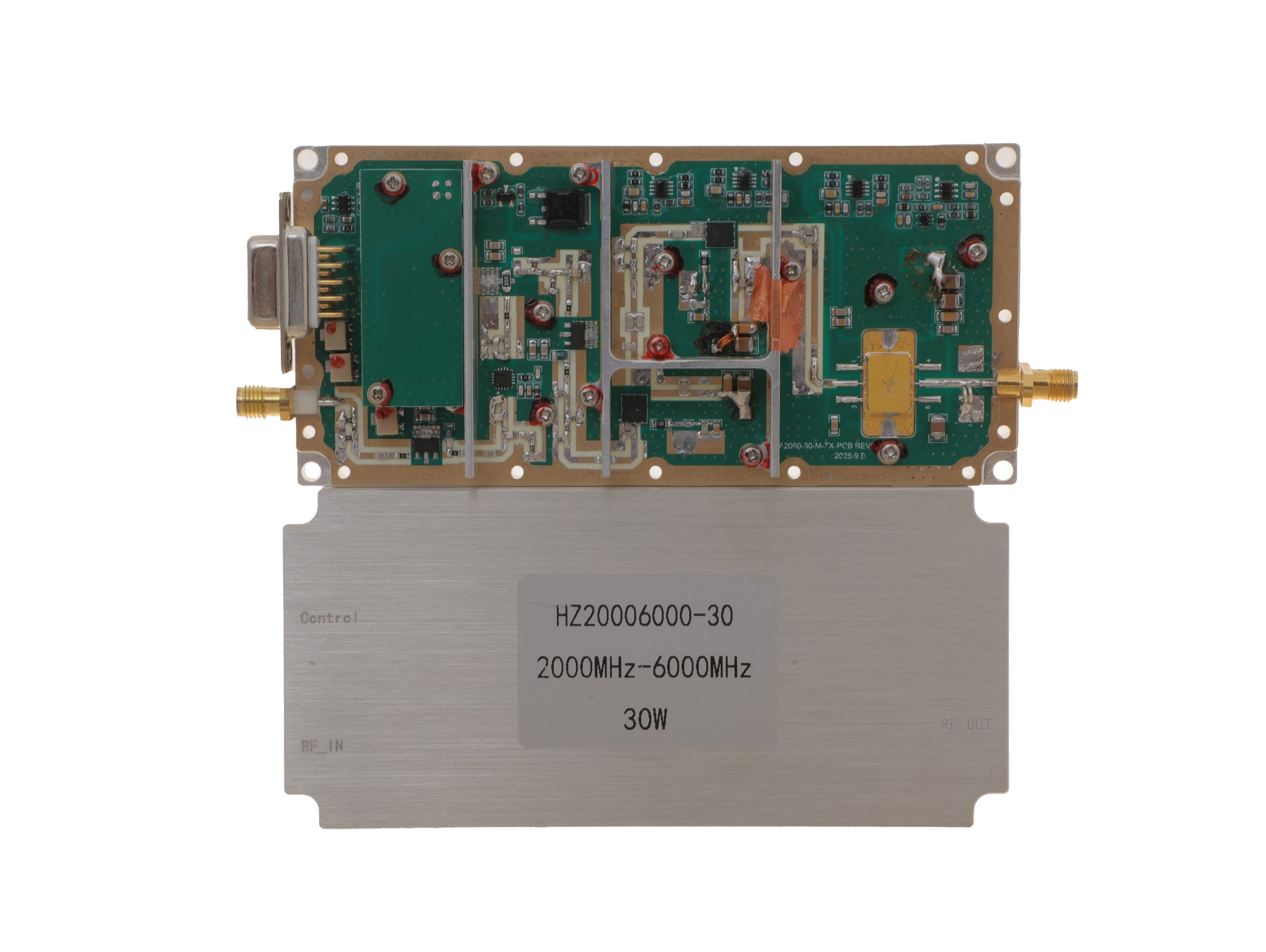 HZ20006000-30NA1Open English PDF ↗ | 25 / 30 W | 3.2 / 4 A | 125 × 59 × 21.5 mm | SMA-KFD46 / SMA-KFD46 | 9-pin D-Sub |
| 50 W | 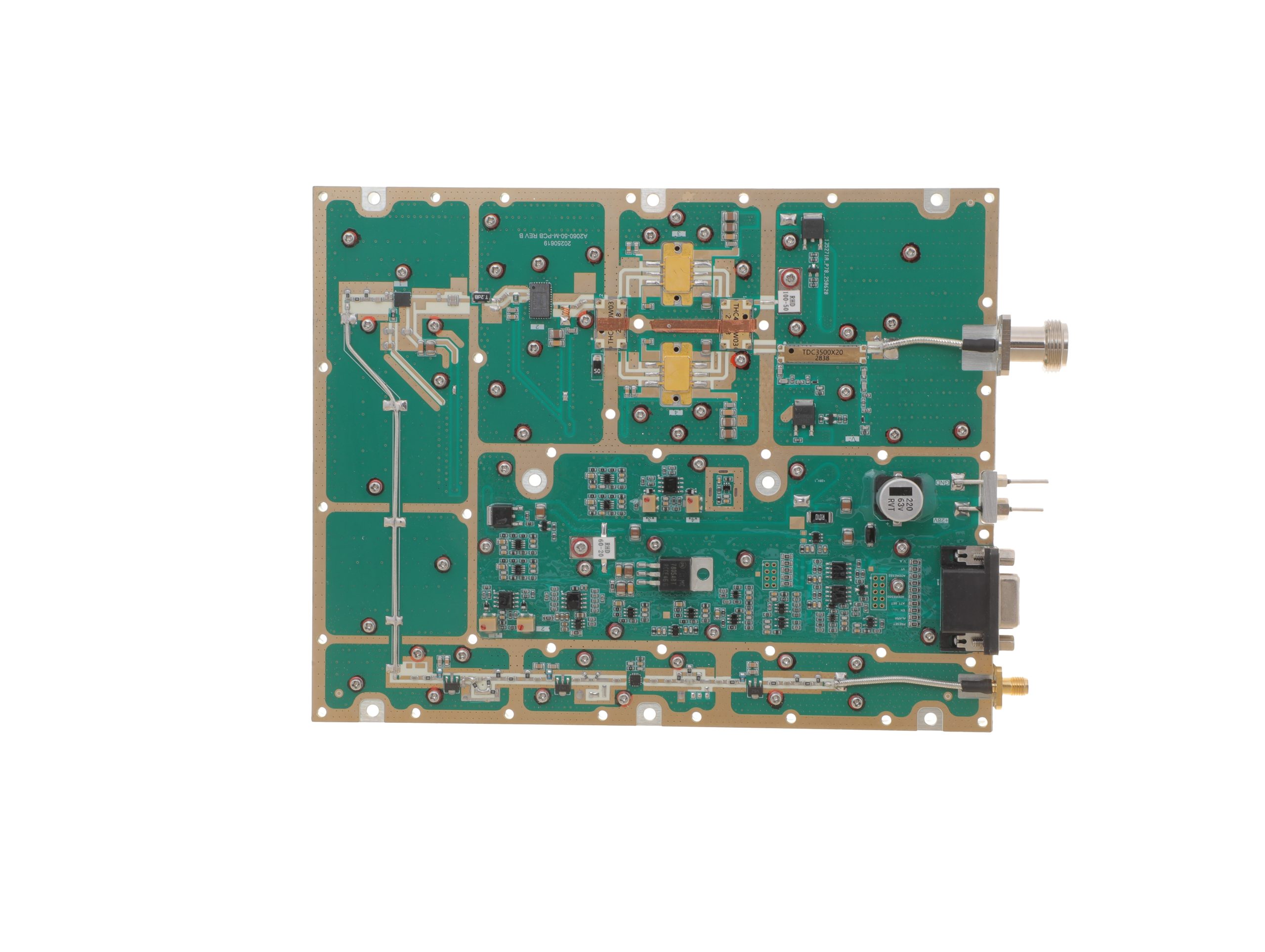 HZ20006000-50NA1Open English PDF ↗ | 40 / 50 W | 10 / 12 A | 200 × 158 × 25 mm | SMA-F / N-F | 15-pin D-Sub |
| 100 W | 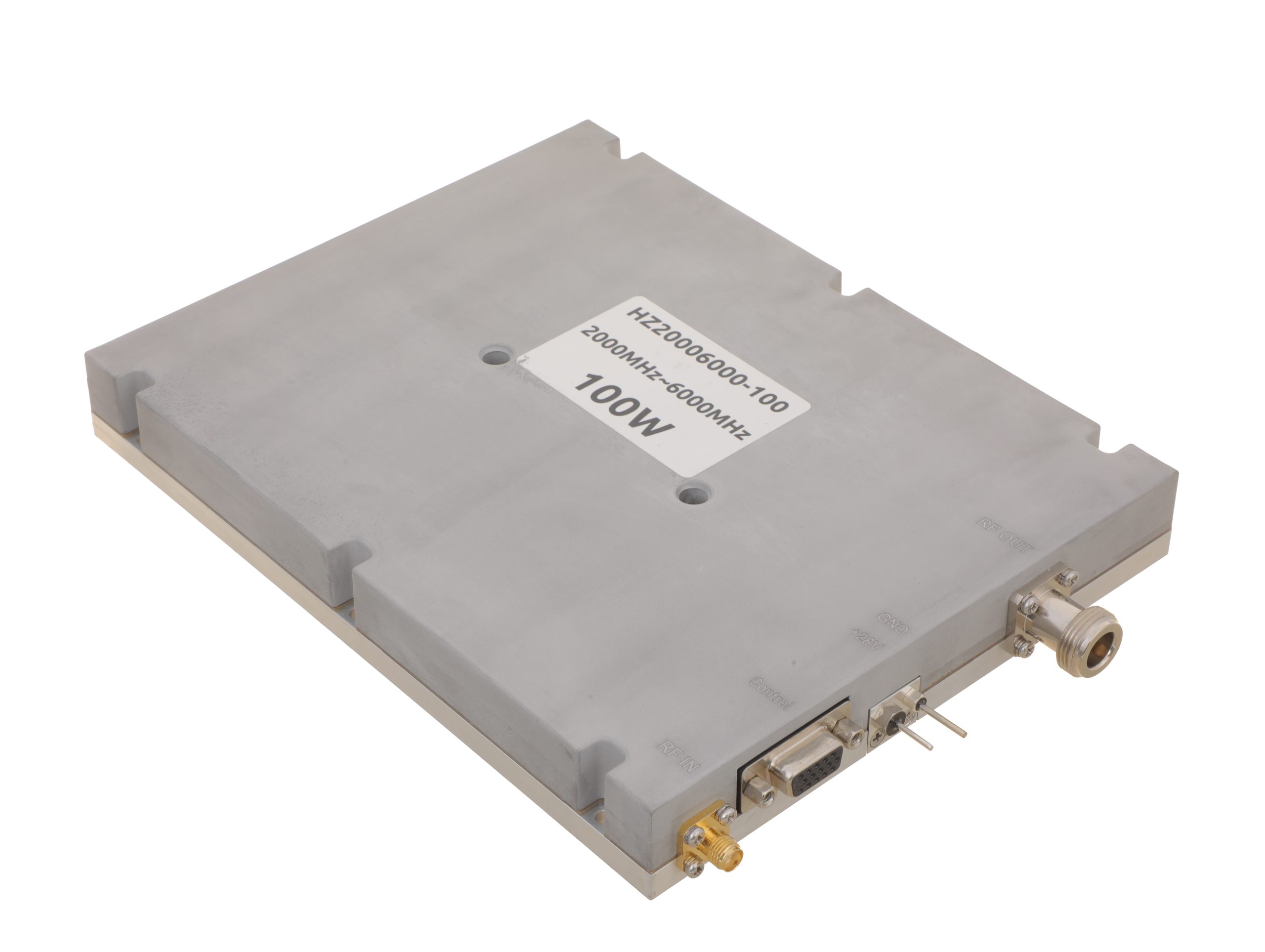 HZ20006000-100NA1Open English PDF ↗ | 80 / 100 W | 19 / 24 A | 200 × 158 × 25 mm | SMA-F / N-F | 15-pin D-Sub |
| 150 W | 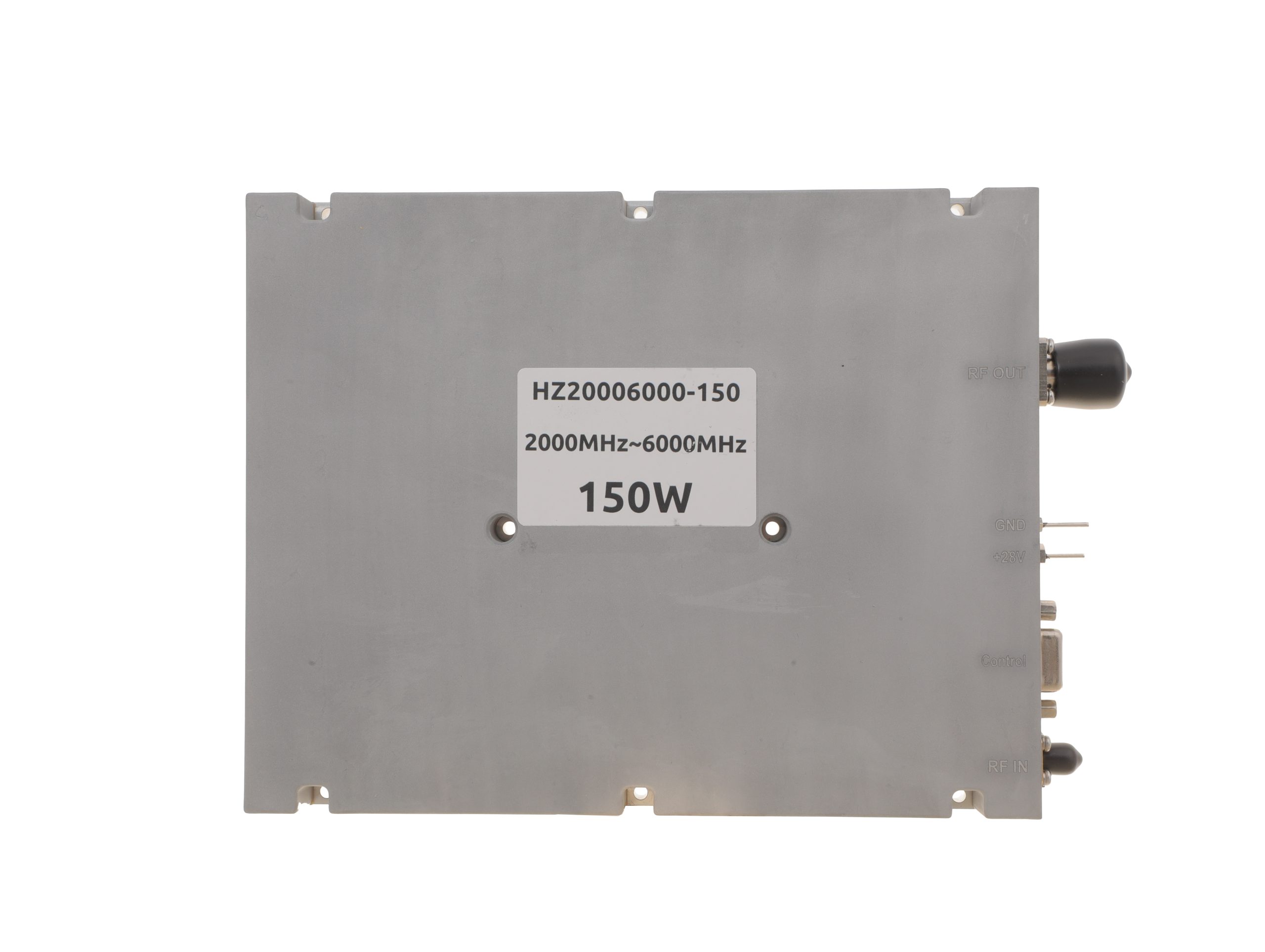 HZ20006000-150NA1Open English PDF ↗ | 120 / 150 W | 22 / 27 A | 200 × 158 × 25 mm | SMA-F / N-F | 15-pin D-Sub |
| 200 W | 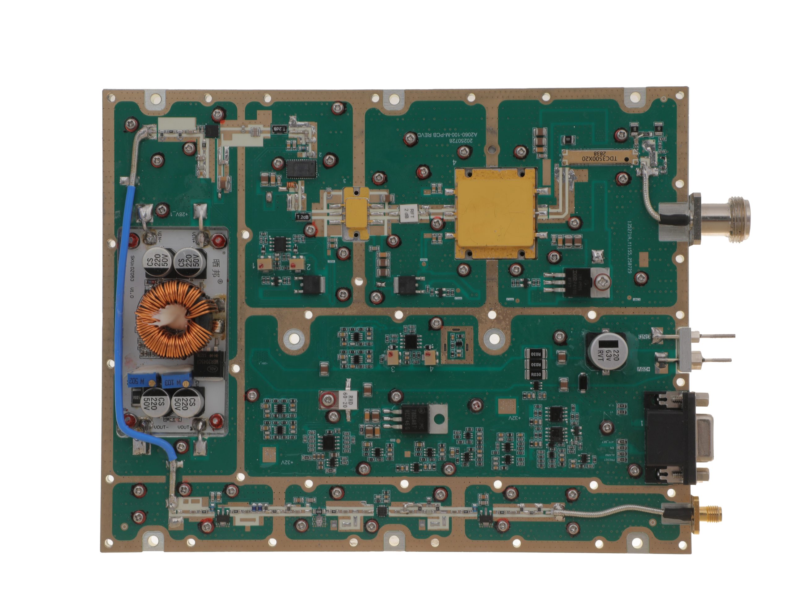 HZ20006000-200NA1Open English PDF ↗ | 160 / 200 W | 29 / 36 A | 280 × 250 × 25 mm | SMA-F / N-F | 15-pin D-Sub |
Review the applicable model’s English PDF datasheet for RF input drive, protection, and optional-function details.
Conclusion
A higher-efficiency PA is cost-justified when verified savings in installed hardware and five-year operating costs cover its price premium, with both candidates meeting the same RF, thermal and availability requirements. The calculation still needs model-specific evidence and matched vendor quotes.
The example’s 600 W PA DC difference is a heat-load and supply-design input, not 600 W of cooling electricity saved. Before selecting a supplier, freeze the RF duty and operating-state schedule, obtain matched PSU, cooling and cabinet prices, and flag every material unpriced TCO item. Engineering and procurement can then review the same cost boundary.
For candidate selection, evaluate RF SKYPOWER’s RF power amplifier module range against a project brief covering frequency, net PA-port output, waveform and duty, concurrent module count, 28 V conditions, load, ambient and mounting limits, annual operating hours, five-year evaluation scope, supply/cooling/cabinet boundaries, currency and required evidence. If comparable model data or quotes are unavailable, submit the same brief for an engineering review; product suitability, documentation and price remain subject to confirmation.