
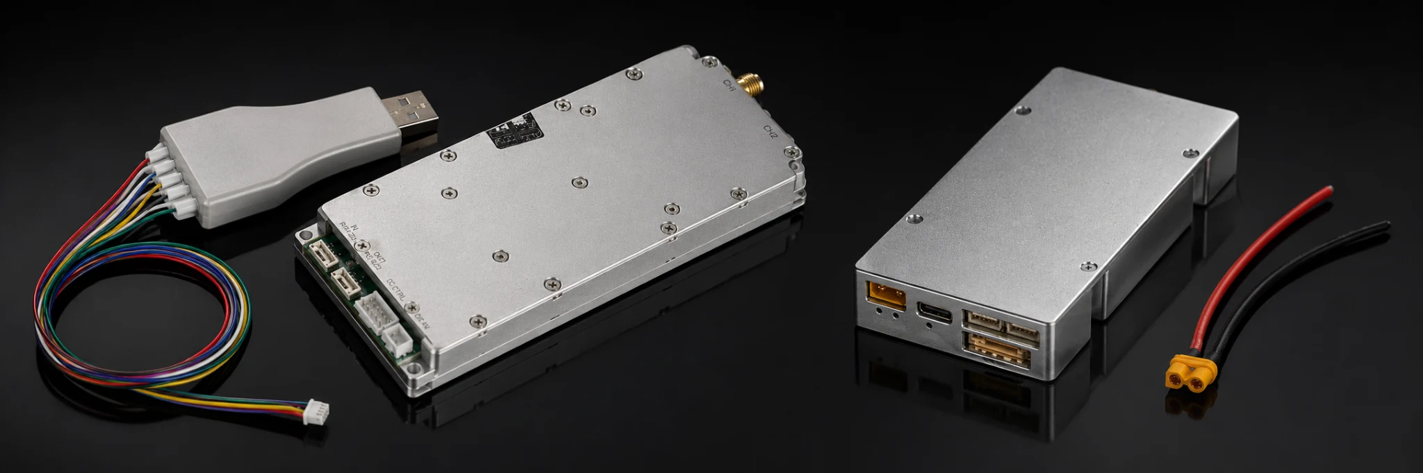


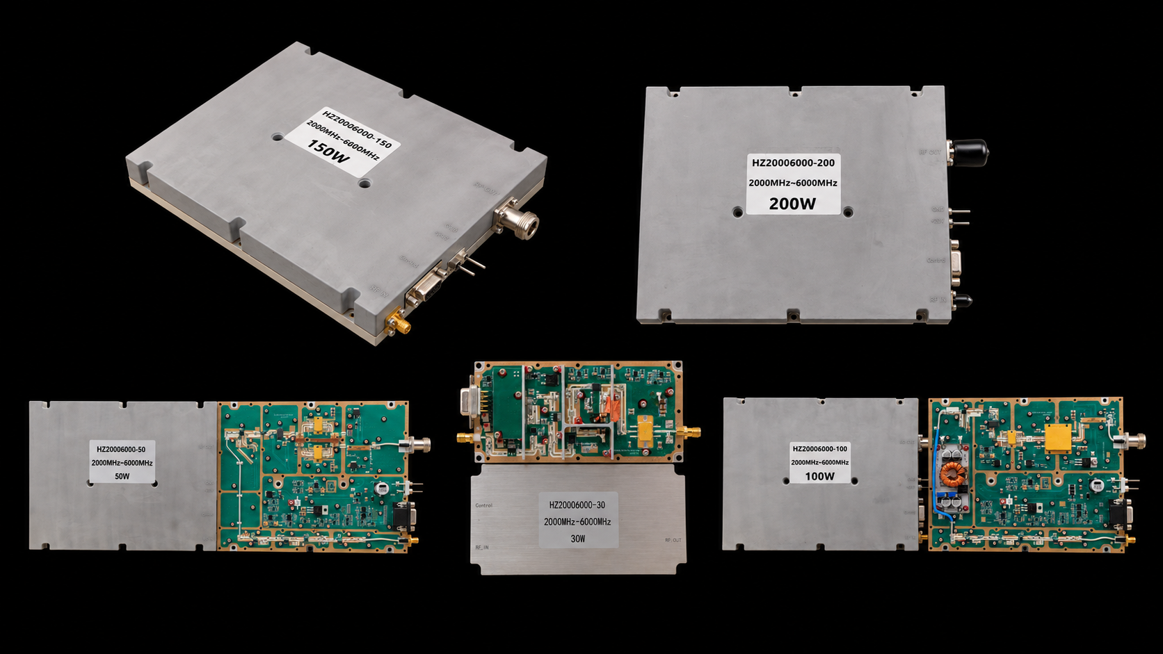
When evaluating 2-6 GHz PA specifications, output wattage alone cannot identify the right module. Start with actual RF drive at the PA input and the waveform your source generates. Then define output power at a clear reference plane and calculate how much power remains after the downstream path.
For this frequency range, the useful engineering chain is:
Source / SDR → actual Pin at the PA input → PA → PA-port Pout → downstream RF-path loss → antenna-end power
The 2–6 GHz range covers several high-frequency RF environments. Applications can include WLAN-related signals, mid-band data links, telemetry, SDR test platforms, and parts of S-band or C-band systems. However, each waveform sets a different operating demand. Common examples include CW, QAM or OFDM, spread-spectrum, frequency-agile, pulsed, and chirped RF.
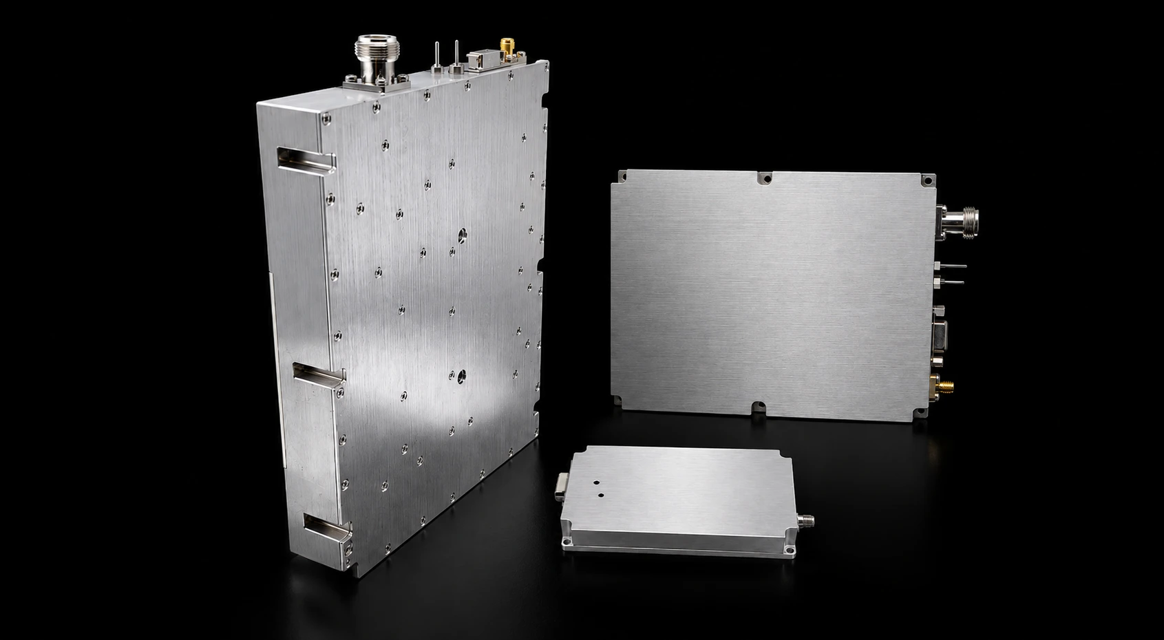
RF SKYPOWER’s current family covers 2000–6000 MHz, up to 200 MHz instantaneous bandwidth, and 30W–200W power classes. To select a model, match those limits to your real RF chain. Check what reaches the PA input, what you need at its output, and what must arrive at the antenna.
1. Why Do 2-6 GHz PA Specifications Need an RF-Chain Budget?
At 2–6 GHz, wattage without a reference plane is not a complete RF requirement.
A practical signal path looks like this:
Source / SDR → PA input → PA output → cable / switch / filter → antenna
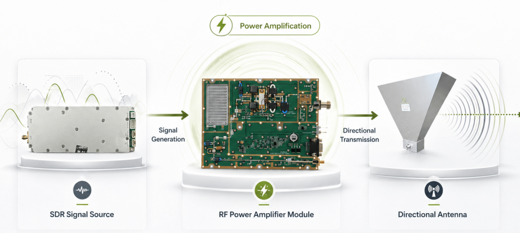
The PA input reference plane is the point at the amplifier input where actual Pin is defined. Actual Pin is the RF power that really reaches that point after the upstream RF path.
The PA-port Pout is the output power referenced to the amplifier output port. Antenna-end power is the power available at the antenna input after the downstream RF path. RF-path loss is the insertion loss introduced by cables, connectors, filters, switches, couplers, and other RF components between those locations.
This method helps because one PA family may work with very different sources. For example, CW, OFDM, frequency-agile, and pulsed signals can share a center frequency. Yet each signal places different demands on drive, bandwidth, linearity, and cooling.
How Do 2-6 GHz PA Specifications Define Reference Planes?
| Reference position | What to define | Main factors | Selection meaning |
|---|---|---|---|
| Signal-source output | Source RF level and waveform | Source setting, waveform, occupied bandwidth | Starting point for the drive budget |
| PA input | Actual Pin | Pre-PA cable, switch, attenuation, filter, and connector loss | Match available drive with Input RF Power Range |
| PA output | PA-port Pout or Psat | Model, drive, frequency, and waveform | Module-level output reference |
| Downstream RF path | Power through the installed path | Cable, connector, filter, switch, coupler, and frequency | Completes the downstream power budget |
| Antenna input | Antenna-end power | PA-port Pout and total downstream loss | Connects PA output with the antenna target |
This reference-plane approach turns a vague request such as “I need a 100W amplifier” into a much more useful engineering requirement: Where must that 100 W be available?
If the answer is “at the PA connector,” the PA-port target leads the selection. If the answer is “at the antenna input,” the PA and downstream RF path need to be considered together.
The same product-boundary logic is part of RF power amplifier module fundamentals: the PA is an RF power-building block inside a larger system rather than the complete RF path. If the project is still deciding whether 2–6 GHz is the right product family, wideband RF power amplifier selection can be used before comparing individual 2–6 GHz power classes.
2. Can Your RF Source Actually Drive the PA?
Once the output reference plane is clear, 2-6 GHz amplifier input power becomes the next selection check: can the source deliver the required drive at the PA input?
A signal generator or SDR may show one output setting, while upstream hardware reduces power before it reaches the PA. Cables, switches, attenuators, and filters can all add loss. Therefore, select the module using actual Pin at the PA input reference plane.
This becomes even more useful when working with different waveform types.
A CW source may be described by a straightforward carrier-power level. An SDR producing QAM or OFDM introduces a varying signal envelope and peak-to-average behavior. A frequency-agile or spread-spectrum source may move through different operating frequencies, while a pulsed source adds peak and duty-cycle considerations.
The source and PA therefore need to be matched as an RF pair rather than selected independently.
The current 30W–200W models also provide different Input RF Power Range options, giving system designers several drive-level choices within the same 2–6 GHz family.
How Do 2-6 GHz PA Specifications Set the Drive Range?
| Power class | Model and datasheet | Input RF Power Range | Psat minimum / typical | Current typical / maximum | Dimensions | RF input / output |
|---|---|---|---|---|---|---|
| 30W | 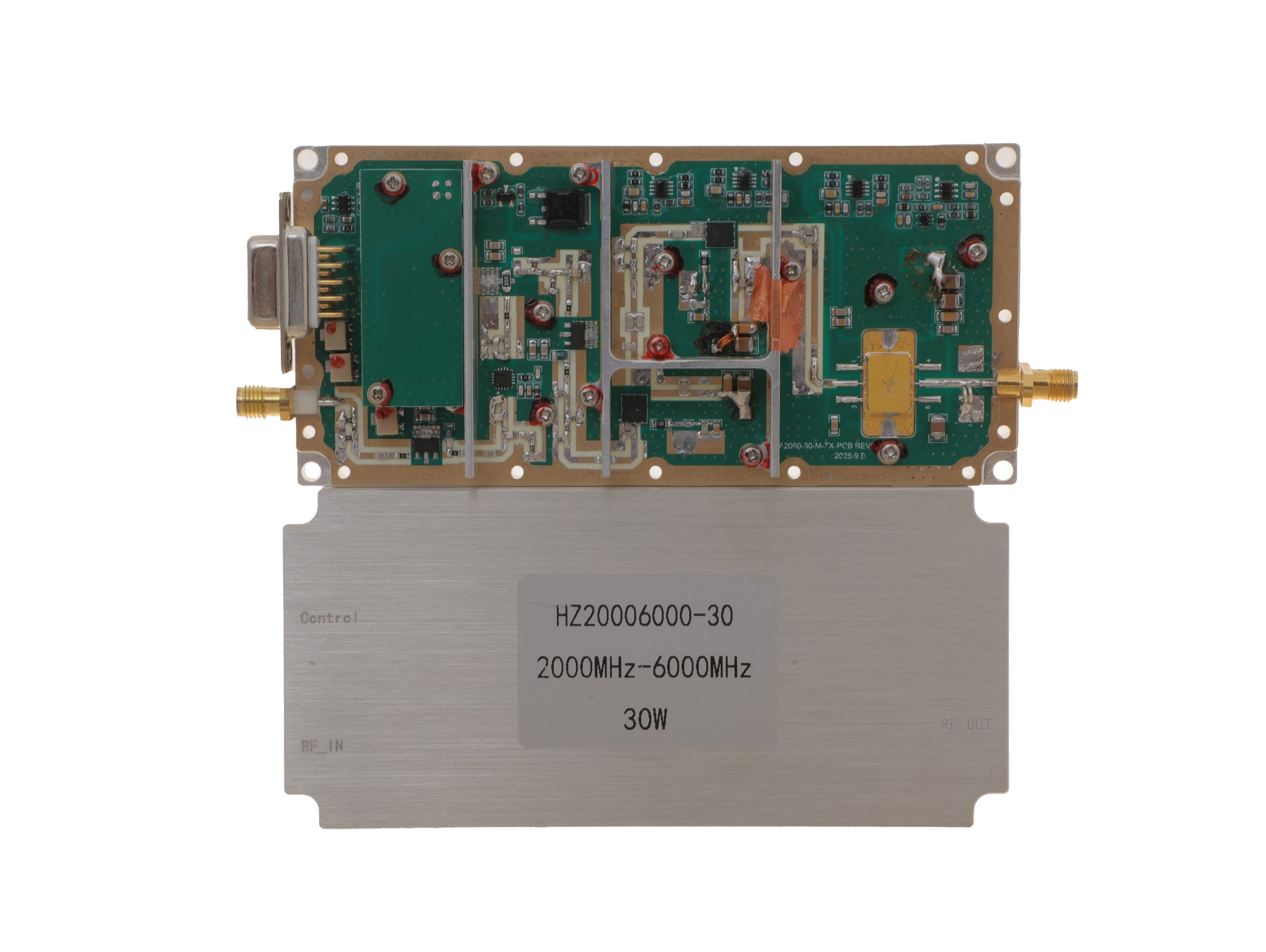 HZ20006000-30NA1 PDF | 0 to +8 dBm | 25 / 30 W | 3.2 / 4 A | 125 × 59 × 21.5 mm | SMA-KFD46 / SMA-KFD46 |
| 50W | 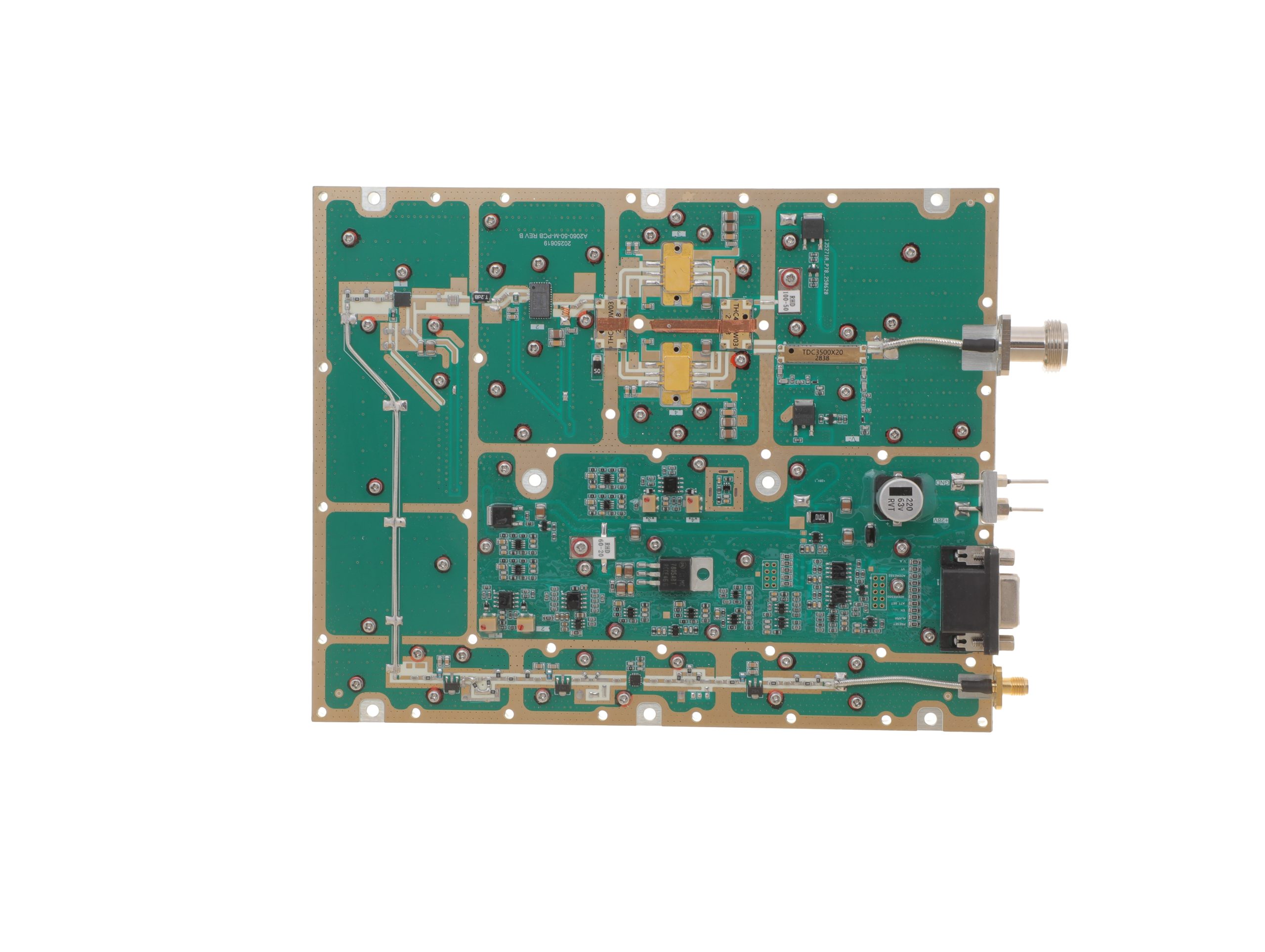 HZ20006000-50NA1 PDF | -10 to +6 dBm | 40 / 50 W | 10 / 12 A | 200 × 158 × 25 mm | SMA-F / N-F |
| 100W | 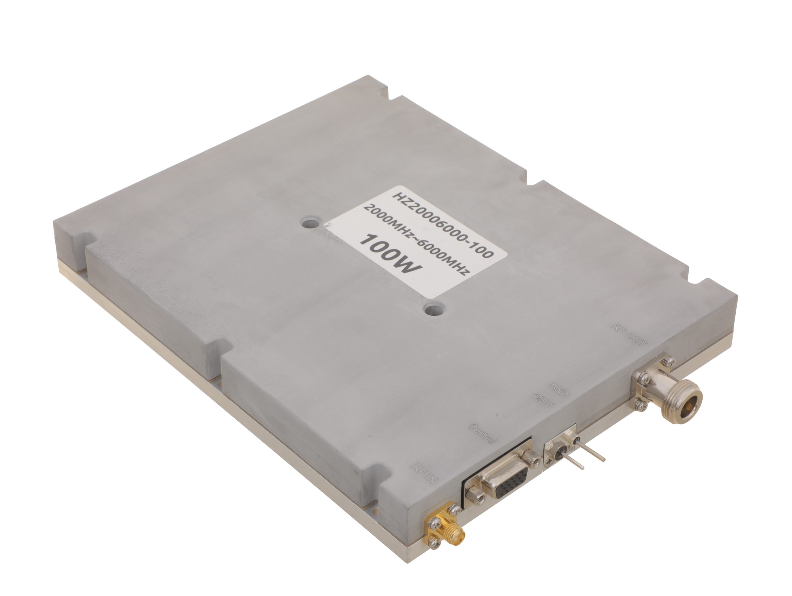 HZ20006000-100NA1 PDF | -7 to +6 dBm | 80 / 100 W | 19 / 24 A | 200 × 158 × 25 mm | SMA-F / N-F |
| 150W | 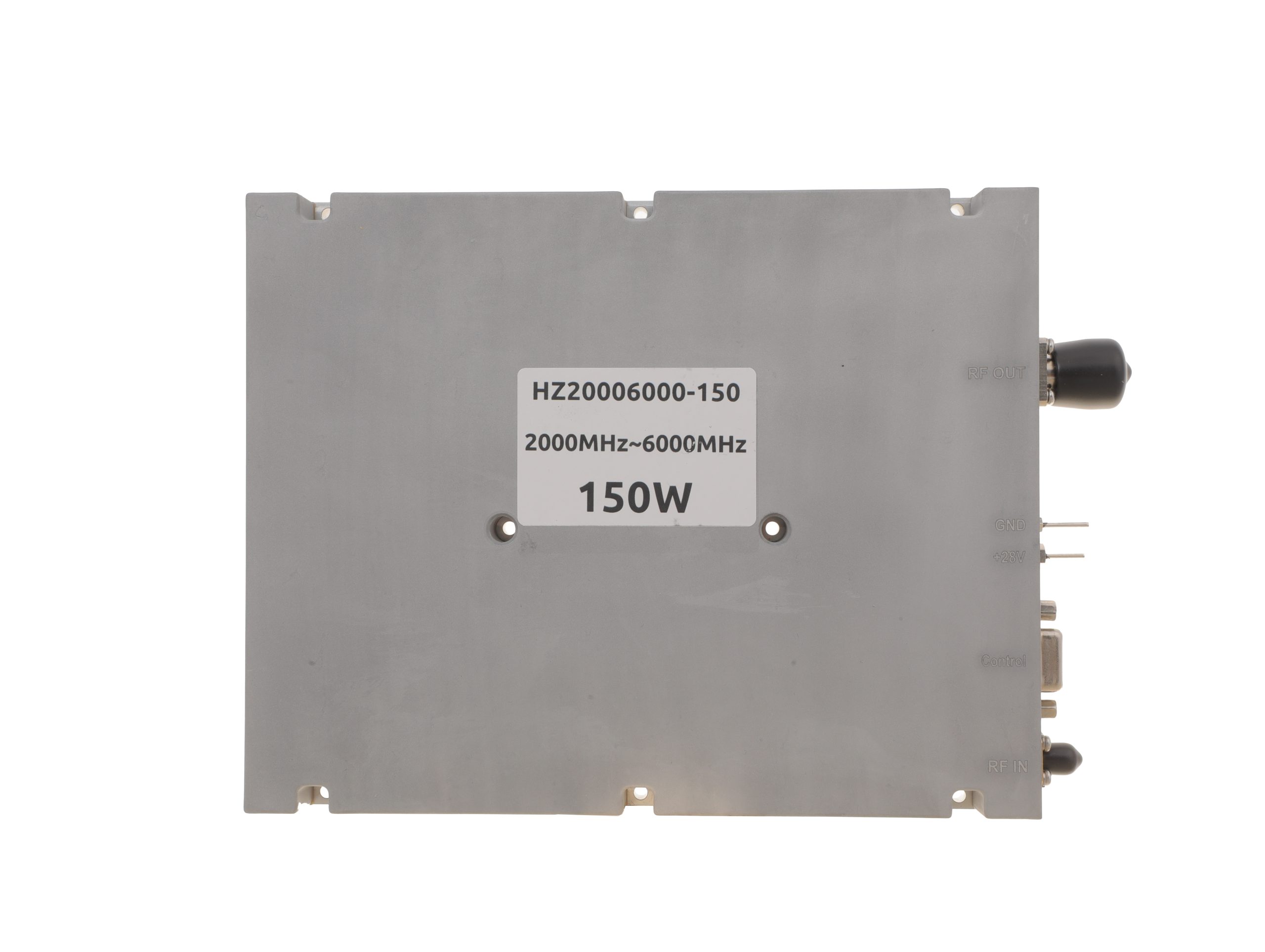 HZ20006000-150NA1 PDF | 0 to +8 dBm | 120 / 150 W | 22 / 27 A | 200 × 158 × 25 mm | SMA-F / N-F |
| 200W | 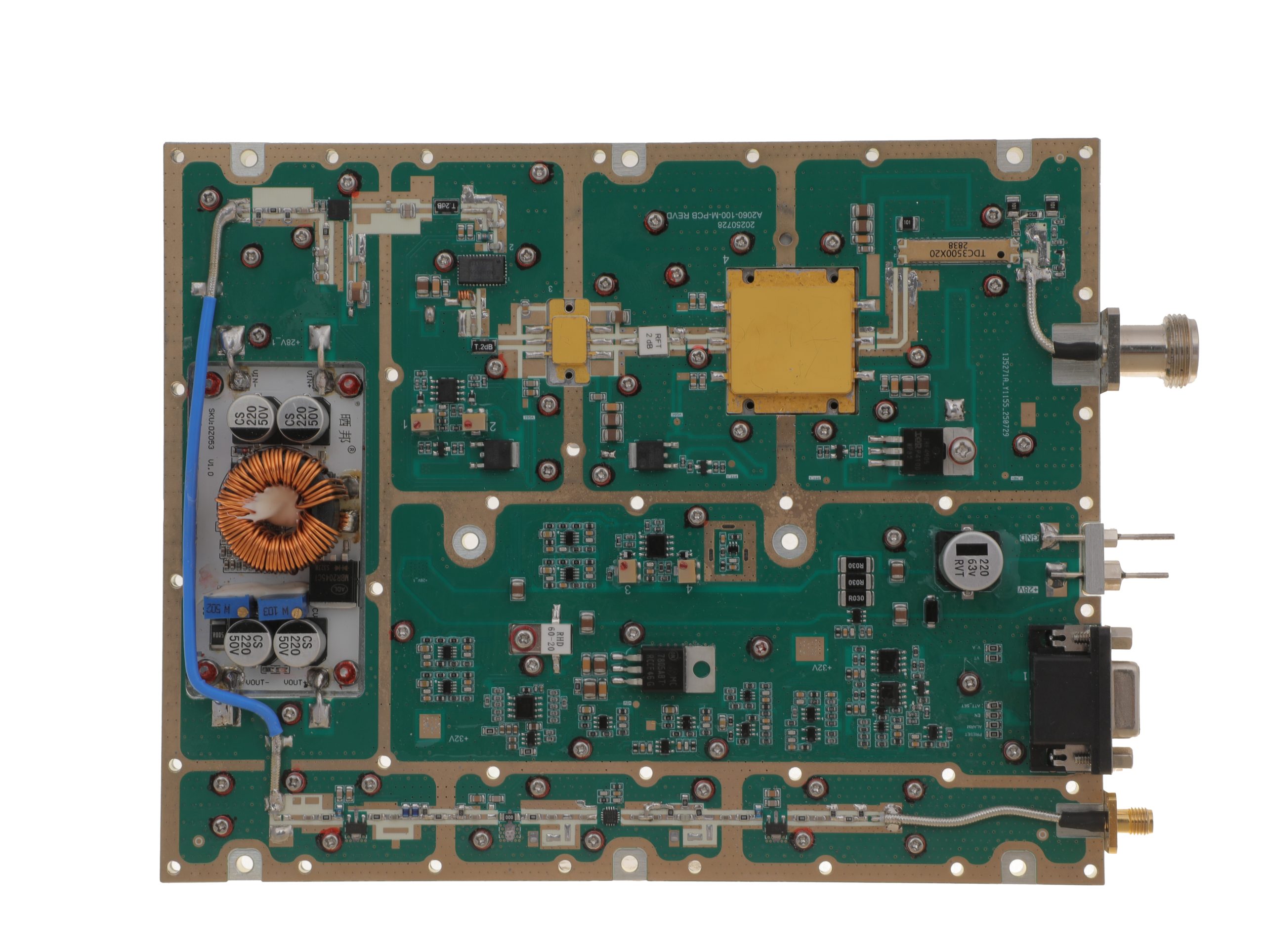 HZ20006000-200NA1 PDF | 0 to +8 dBm | 160 / 200 W | 29 / 36 A | 280 × 250 × 25 mm | SMA-F / N-F |
The drive range is a useful first filter. For example, the 50W and 100W models provide lower published input-range floors than the 150W and 200W versions, which can matter when the upstream source or RF path has limited available drive.
Small-signal Gain provides another useful module parameter, but it serves a different purpose from full-power operation. The practical selection method is to compare the project’s actual available Pin with the published Input RF Power Range instead of trying to derive the required drive from Psat and small-signal Gain alone.
Once actual Pin, frequency, bandwidth, and output requirement are defined, the current 2-6 GHz RF power amplifier family provides 30W, 50W, 100W, 150W, and 200W options for model comparison.
3. PA-Port Pout Is Not Antenna-End Power
For 2-6 GHz antenna-end power planning, PA-port Pout and antenna input power should be treated as two reference points in the same RF budget.
The PA generates its RF output at the amplifier output connector. From there, the signal may still pass through cable, connectors, filters, switches, couplers, or other RF hardware before reaching the antenna.
The useful relationship is:
PA-port Pout → downstream RF-path loss → antenna-end power
That distinction is valuable because it lets the designer choose the PA power class from the actual system target instead of simply choosing the same wattage written in the antenna requirement.
Suppose the system requirement is defined at the antenna input. The required PA-port Pout then needs to leave enough power budget for the downstream path. If the requirement is already defined at the PA output connector, the model can be compared directly at that reference plane.
Waveform belongs in the same power review. A CW Psat value provides a module-level output reference. By contrast, a broadband signal also needs enough linear range for its changing envelope. For OFDM or QAM, check peak-to-average behavior and occupied bandwidth alongside nominal wattage.
The core selection idea remains simple: define the power at the PA output and the power required at the antenna as separate values.
For installations where cable loss, antenna matching, reflected power, or installed-path VSWR becomes a major part of the decision, RF-path, cable, antenna, and VSWR behavior can be reviewed together with the amplifier selection.
4. How RF-Path Loss Changes the Power Budget at 2–6 GHz
RF-path loss works on both sides of the PA.
Before the amplifier:
Source → cable / switch / attenuator / filter → actual Pin
This side determines how much source power actually reaches the amplifier.
After the amplifier:
PA-port Pout → connector / cable / filter / switch → antenna-end power
This side determines how much amplified RF power remains available toward the antenna.
Keeping those two path sections separate makes the power budget much easier to use. The pre-PA path helps answer “Can I drive this model?” while the post-PA path helps answer “How much power reaches the final RF load?”
At 2–6 GHz, path loss can change with frequency. For example, the same cable and switch path may have different loss at 2.4 GHz and 5.8 GHz. Therefore, use loss data from each required operating point.
Signal bandwidth can matter as well. For a narrow CW carrier, the path condition at one operating frequency may dominate the calculation. For a broadband signal such as OFDM or another spread-spectrum waveform, the designer may also care about the RF path across the occupied signal bandwidth.
For the current 2–6 GHz family, RF power amplifier instantaneous bandwidth is specified at up to 200 MHz, giving broadband SDR and digitally generated RF architectures useful signal-width headroom. The installed cable, filter, switch, and antenna path should then be selected to complement the bandwidth and frequencies the project actually intends to use.
For PA selection, the most useful project inputs are therefore the pre-PA loss, downstream loss, and the important operating frequencies. Once those are known, the source drive, PA power class, and antenna-end target can all be placed in the same RF budget.
5. Which 2-6 GHz PA Specifications Change from 30W to 200W?
Moving from 30W to 200W is not simply a wattage upgrade. The input-drive boundary, DC demand, mechanical platform, and RF interface also change across the family.
The 30W model uses the smallest platform with SMA input and output connectors. From 50W upward, models use a larger platform with SMA input and N-type output. Meanwhile, the 200W model needs a larger enclosure. DC demand also rises with power, so check supply capacity, cooling, and installation space.
Input-drive requirements vary between power classes as well. The actual Pin available from the source and upstream RF path should therefore be matched to the selected model rather than assumed to remain the same when moving to a higher output level.
The current models also specify a 1 μs PA Enable/Disable response, providing fast module-level RF on/off control for gated or timed transmission.
6. What the Datasheet Can Tell You About a 2–6 GHz Module
A current RF amplifier module datasheet gives the engineer the RF, DC, mechanical, and interface data needed for an initial 2–6 GHz shortlist.
The current model specifications provide key fields including:
- 2000–6000 MHz operating frequency
- 200 MHz maximum instantaneous bandwidth
- Input RF Power Range
- Psat
- small-signal Gain
- Input VSWR
- operating voltage and current
- mechanical dimensions
- RF input and output connectors
- PA Enable/Disable timing
Together, these parameters describe much more than “2–6 GHz + watts.”
Frequency range tells you where the PA can operate. Meanwhile, the 200 MHz instantaneous-bandwidth limit matters for broadband digital and SDR signals. OFDM, for example, can occupy far more bandwidth than one CW carrier.
Input RF Power Range shows whether your source and upstream path can drive a model. Next, Psat defines its module-level output class. Current and dimensions then set supply, cooling, enclosure, and mounting needs.
For example, gain-compression testing checks where amplifier gain drops as input power rises. This measurement helps you compare output at a defined drive level rather than relying on a wattage label alone.
RF connectors also become more significant as the power class rises. The 30W platform uses SMA-KFD46 at the RF input and output, while the 50W–200W models use SMA-F input and N-F output, giving the higher-power platforms a different physical integration arrangement.
Which 2-6 GHz PA Specifications Change with the Waveform?
CW and narrowband RF place more weight on output power, drive, current, and thermal integration.
QAM and OFDM require enough instantaneous bandwidth and linear operating range for their changing envelope.
Frequency-agile or spread-spectrum signals need suitable drive and RF-path behavior across every required operating point.
Pulsed or chirped RF adds duty cycle, peak power, pulse conditions, bandwidth, and control timing to the project definition.
The datasheet therefore gives the PA-level building blocks for the decision. The project RF path adds the final information needed to connect those specifications to actual Pin and antenna-end power.
7. Standard Module, RF-Path Review, or Custom Engineering?
Once the waveform, actual Pin, output reference plane, and RF path are understood, the next route becomes much easier to choose.
Standard 2–6 GHz Module
A standard module fits when your frequency falls within 2–6 GHz and signal bandwidth stays below 200 MHz. You also need enough actual Pin and a clear PA-port Pout target. Finally, confirm DC, cooling, mechanical, and RF interface limits.
The current standard family provides 30W, 50W, 100W, 150W, and 200W classes, allowing the designer to scale RF output while remaining within the same 2–6 GHz product family.
The 2000–6000 MHz RF power amplifier range is the direct route for comparing those standard options and their current specifications.
RF-Path Review
An RF-path review becomes useful when the PA itself is understood but the remaining question is how much power reaches the antenna.
Typical items include cable and connector loss, filters, switches, couplers, feeder conditions, installed-path VSWR, and reflected power.
In this case, the goal is not simply to move to a larger PA. It is to build the cleanest possible relationship between PA-port Pout and antenna-end power. The RF path, cable, antenna, and VSWR review provides the natural next engineering layer.
Custom Engineering
Custom engineering becomes relevant when the project needs something outside the standard combination of frequency, output power, input drive, RF interface, mechanical platform, cooling, control, or project-specific evidence.
Waveform requirements can also be part of that discussion. An SDR-driven broadband signal, a special duty-cycle requirement, a frequency-agile architecture, or a project with unique control timing may need a more detailed engineering review around the standard module boundary.
A custom RF power amplifier RFQ can start from the project’s actual frequency points, waveform, bandwidth, available Pin, PA-port Pout target, antenna-end target, RF-path components, DC supply, cooling, mechanics, connectors, and control requirements.
| Project condition | Best next route | Information to prepare |
|---|---|---|
| Standard frequency, drive, output, and interfaces | Compare standard 2–6 GHz modules | Frequency points, waveform, Pin, Pout, DC, and cooling |
| Uncertain cable, filter, switch, antenna, or VSWR loss | Request an RF-path review | Installed path, component loss, load, and reference planes |
| Requirements outside a standard model boundary | Request custom engineering | RF, mechanical, thermal, control, test, and quantity needs |
8. What Should You Confirm Before Ordering?
Before ordering a 2–6 GHz RF power amplifier, confirm every reference plane in the complete RF chain:
Source / waveform → actual Pin → PA → PA-port Pout → downstream RF-path loss → antenna-end power
The current family covers 2000–6000 MHz, up to 200 MHz instantaneous bandwidth, and five power classes from 30W through 200W. It also specifies a 1 μs PA Enable/Disable response. Together, these limits help you screen modules for CW, broadband, modulated, or frequency-agile systems.
The framework can help determine the appropriate power class, source-drive requirement, RF-path budget, and next integration route. The final antenna-end result still depends on the project’s actual downstream cable, connectors, switches, filters, and other installed RF-path conditions.
The main point to keep clear is the reference plane: a 100W PA specification describes PA-port output, while the antenna-end target belongs to the complete RF path. In the same way, the useful input value is the RF power that actually reaches the PA input rather than only the source setting.
Before final model selection, define the waveform, operating frequency, maximum instantaneous bandwidth, actual Pin, required PA-port Pout, downstream RF path, antenna-end target, DC supply, mechanical space, RF interfaces, and cooling conditions.
With those inputs in hand, compare the current 2000–6000 MHz RF power amplifier models. If the main remaining task is cable, connector, switch, filter, VSWR, or antenna-path integration, move into the RF-path review. If the standard frequency, power, drive, mechanical, cooling, interface, control, or waveform conditions need to be adapted, submit them through the RF SKYPOWER RFQ for engineering review.